CG Propensity

CG has tasked me with developing a predictive model utilizing the “Space Pirates” game data. The primary objective is to identify which gamers are more or less inclined to purchase the “Zalon” campaign. This involves analyzing player behavior, engagement levels, and other relevant metrics to forecast their purchasing decisions accurately.

Analytical Models Employed:

To achieve the objective, the following predictive analytics models are being considered and implemented throughout the campaign:

• Logistic Regression Model: This model is used for binary classification tasks. In this context, it will predict the likelihood of a gamer purchasing the Zalon campaign, categorizing predictions into two groups: likely buyers and unlikely buyers.

• Neural Network Model: This model, known for its ability to capture complex nonlinear relationships, is employed to understand deeper patterns in gamer behavior that may influence their decision to purchase. It leverages layers of processing units to learn from the data, offering a more nuanced prediction compared to traditional models.

• Random Forest Model: A robust ensemble learning method that uses multiple decision trees to make predictions. It is particularly useful for handling large datasets with numerous variables, providing insights into the importance of different features affecting the purchasing decision.

Each of these models offers unique strengths in data analysis and prediction accuracy. By comparing their performance, we aim to identify the most effective approach to predict gamer behavior regarding the Zalon campaign purchase decision.

import matplotlib as mpl
import matplotlib.pyplot as plt
import pandas as pd
import pyrsm as rsm 
import numpy as np 
from scipy import stats
from sklearn.preprocessing import power_transform

# load a custom python module
#from utils.functions import example


## setup functions for autoreload
#%reload_ext autoreload
#%autoreload 2
#%aimport utils.functions

Data Description

## loading the data
cg_organic = pd.read_parquet("./data/cg_organic.parquet")

Creative gaming

Game telemetry dataset used for the Creative Gaming: Propensity-to-Buy Modeling case

Feature descriptions

• converted: Purchased the Zalon campain (“yes” or “no”)
• GameLevel: Highest level of game achieved by the user
• NumGameDays: Number of days user played the game in last month (with or without network connection)
• NumGameDays4Plus: Number of days user played the game in last month with 4 or more total users (this implies using a network connection)
• NumInGameMessagesSent: Number of in-game messages sent to friends
• NumFriends: Number of friends to which the user is connected (necessary to crew together in multiplayer mode)
• NumFriendRequestIgnored: Number of friend requests this user has not replied to since game inception
• NumSpaceHeroBadges: Number of “Space Hero” badges, the highest distinction for gameplay in Space Pirates
• AcquiredSpaceship: Flag if the user owns a spaceship, i.e., does not have to crew on another user’s or NPC’s space ship (“no” or “yes”)
• AcquiredIonWeapon: Flag if the user owns the powerful “ion weapon” (“no” or “yes”)
• TimesLostSpaceship: The number of times the user destroyed his/her spaceship during gameplay. Spaceships need to be re-acquired if destroyed.
• TimesKilled: Number of times the user was killed during gameplay
• TimesCaptain: Number of times in last month that the user played in the role of a captain
• TimesNavigator: Number of times in last month that the user played in the role of a navigator
• PurchasedCoinPackSmall: Flag if the user purchased a small pack of Zathium in last month (“no” or “yes”)
• PurchasedCoinPackLarge: Flag if the user purchased a large pack of Zathium in last month (“no” or “yes”)
• NumAdsClicked: Number of in-app ads the user has clicked on
• DaysUser: Number of days since user established a user ID with Creative Gaming (for Space Pirates or previous games)
• UserConsole: Flag if the user plays Creative Gaming games on a console (“no” or “yes”)
• UserHasOldOS: Flag if the user has iOS version 10 or earlier (“no” or “yes”)
• rnd_30k: Dummy variable that randomly selects 30K customers (1) and the remaining 90K (0)

Part 1

cg_organic["converted_yes"] = cg_organic["converted"].map({"yes": 1, "no": 0})

We want to turn the yes’s and no’s into integers to allow for us to take the average of the converted column and calculate the average probability of converting. To do this, we use the map function to map the yes’s and no’s numerically represent.

What is the probability of organically converting to Zalon

#prob_converting = cg_organic["converted_1_0"].mean()
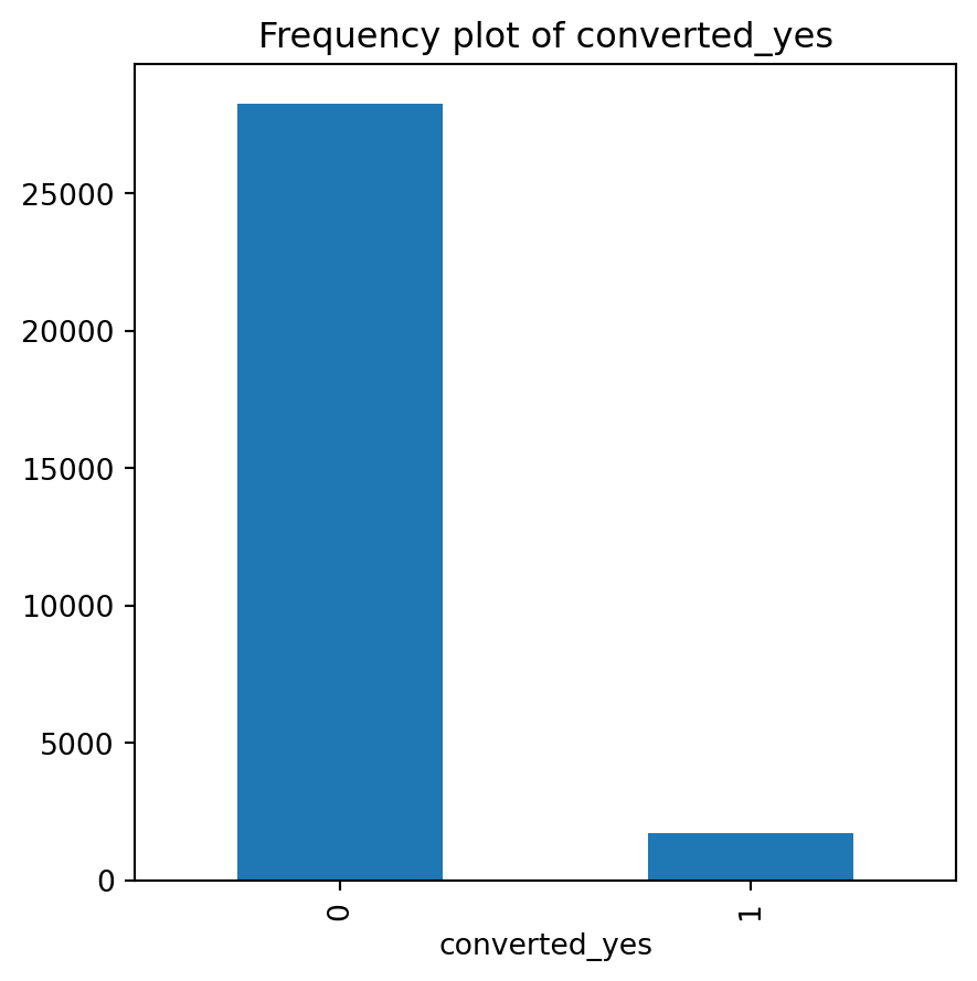
prob_converting = cg_organic["converted"].value_counts(normalize=True)
prob_converting = prob_converting["yes"]
print(prob_converting)

0.05753333333333333

We can find the probability of organically converting to Zalon by taking the average of the coverted_yes column in the cq_organic cg_organicbase. This probability is 5.8%.

Basic summary statistics for each feature

cg_organic.info()

<class 'pandas.core.frame.DataFrame'>
Index: 30000 entries, 34184 to 51934
Data columns (total 22 columns):
 #   Column                   Non-Null Count  Dtype   
---  ------                   --------------  -----   
 0   converted                30000 non-null  category
 1   GameLevel                30000 non-null  int32   
 2   NumGameDays              30000 non-null  int32   
 3   NumGameDays4Plus         30000 non-null  int32   
 4   NumInGameMessagesSent    30000 non-null  int32   
 5   NumSpaceHeroBadges       30000 non-null  int32   
 6   NumFriendRequestIgnored  30000 non-null  int32   
 7   NumFriends               30000 non-null  int32   
 8   AcquiredSpaceship        30000 non-null  category
 9   AcquiredIonWeapon        30000 non-null  category
 10  TimesLostSpaceship       30000 non-null  int32   
 11  TimesKilled              30000 non-null  int32   
 12  TimesCaptain             30000 non-null  int32   
 13  TimesNavigator           30000 non-null  int32   
 14  PurchasedCoinPackSmall   30000 non-null  category
 15  PurchasedCoinPackLarge   30000 non-null  category
 16  NumAdsClicked            30000 non-null  int32   
 17  DaysUser                 30000 non-null  int32   
 18  UserConsole              30000 non-null  category
 19  UserHasOldOS             30000 non-null  category
 20  training                 30000 non-null  int32   
 21  converted_yes            30000 non-null  category
dtypes: category(8), int32(14)
memory usage: 2.1+ MB

Using the cg_organic.info() code, we are able to populate a summary overview of the variables that are present in the cq_organic database. As we can see, there seems to be no missing values, which allows us to begin our exploratory analytics right away without needing to conduct cg_organic cleaning. In addition, info output provides an overview of what type of variable each of the columns are, enabling us to manipulate the types if needed. For example, we created a new column called converted_yes to calculate the average conversion rate of cg gaming organic users.

cg_organic.describe()

	GameLevel	NumGameDays	NumGameDays4Plus	NumInGameMessagesSent	NumSpaceHeroBadges	NumFriendRequestIgnored	NumFriends	TimesLostSpaceship	TimesKilled	TimesCaptain	TimesNavigator	NumAdsClicked	DaysUser	training
count	30000.000000	30000.000000	30000.000000	30000.000000	30000.000000	30000.000000	30000.000000	30000.000000	30000.000000	30000.000000	30000.000000	30000.000000	30000.000000	30000.000000
mean	6.246733	12.241400	1.257267	73.777400	0.443933	29.589100	47.733833	4.435567	0.293400	1.583033	1.403967	9.494600	2626.371933	0.700000
std	2.774055	7.097305	3.191210	107.441593	1.517762	33.990783	94.329939	11.546392	3.415129	8.770534	7.950200	7.395841	661.428007	0.458265
min	1.000000	1.000000	0.000000	0.000000	0.000000	0.000000	0.000000	0.000000	0.000000	0.000000	0.000000	0.000000	244.000000	0.000000
25%	4.000000	6.000000	0.000000	0.000000	0.000000	0.000000	0.000000	0.000000	0.000000	0.000000	0.000000	4.000000	2162.000000	0.000000
50%	7.000000	13.000000	0.000000	26.000000	0.000000	16.000000	5.000000	0.000000	0.000000	0.000000	0.000000	8.000000	2557.000000	1.000000
75%	9.000000	18.000000	0.000000	112.000000	0.000000	53.000000	43.000000	4.000000	0.000000	0.000000	0.000000	12.000000	3105.000000	1.000000
max	10.000000	28.000000	24.000000	1227.000000	12.000000	121.000000	486.000000	298.000000	178.000000	429.000000	545.000000	38.000000	4139.000000	1.000000

# Non-numeric columns
non_numeric_columns = cg_organic.select_dtypes(include=['object', 'category']).columns

# Find the number of Distinct values in each column
cg_organic[non_numeric_columns].nunique()

converted                 2
AcquiredSpaceship         2
AcquiredIonWeapon         2
PurchasedCoinPackSmall    2
PurchasedCoinPackLarge    2
UserConsole               2
UserHasOldOS              2
converted_yes             2
dtype: int64

# Find the most common levels in each column
cg_organic[non_numeric_columns].apply(lambda x: x.value_counts().idxmax())

converted                  no
AcquiredSpaceship          no
AcquiredIonWeapon          no
PurchasedCoinPackSmall     no
PurchasedCoinPackLarge     no
UserConsole               yes
UserHasOldOS               no
converted_yes               0
dtype: object

Generate histograms for all numeric variables and frequency plots for non numeric variables

cg_organic.hist(figsize=(15, 15))

array([[<Axes: title={'center': 'GameLevel'}>,
        <Axes: title={'center': 'NumGameDays'}>,
        <Axes: title={'center': 'NumGameDays4Plus'}>,
        <Axes: title={'center': 'NumInGameMessagesSent'}>],
       [<Axes: title={'center': 'NumSpaceHeroBadges'}>,
        <Axes: title={'center': 'NumFriendRequestIgnored'}>,
        <Axes: title={'center': 'NumFriends'}>,
        <Axes: title={'center': 'TimesLostSpaceship'}>],
       [<Axes: title={'center': 'TimesKilled'}>,
        <Axes: title={'center': 'TimesCaptain'}>,
        <Axes: title={'center': 'TimesNavigator'}>,
        <Axes: title={'center': 'NumAdsClicked'}>],
       [<Axes: title={'center': 'DaysUser'}>,
        <Axes: title={'center': 'training'}>, <Axes: >, <Axes: >]],
      dtype=object)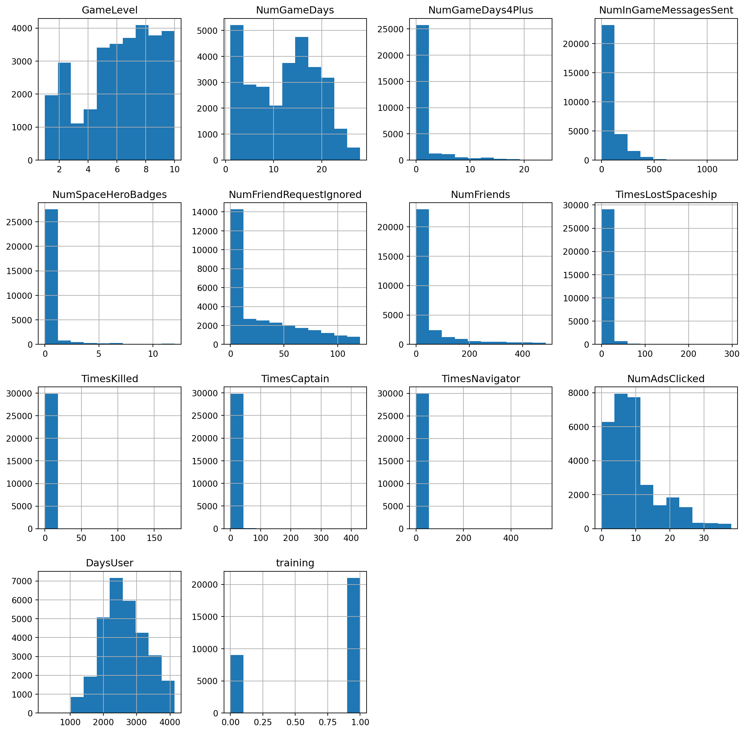

The histograms above show the distribution of each variable present in our dataset. This is a critical step within the data preprocessing part of building a model. We can use the distributions to identify skew in our variables, and transform the variables so they are normally distributed.

From the histogram above, we see many variables in this dataset are heavily skewed to the left. DaysUser and GameLevel are the only variables with a slight right skew. Because of the skews in the variables, this will give us an inaccurate model if we were to use the variables with their current distributions. Therefore, we need to transform the variables based on the skew they are exhibiting in the histograms. To correct the heavy left skew that is present in DaysUser and GameLevel, Before we begin building any models, we will want to transform these variables.

Because of the heavy skew present in the columns in the data, we will want to transform them to normalize their distribution. Logistic regression does not assume a normal distribution of the independent variables, however, transformations can still help in stabilizing the variance and making relationships more linear. Therefore, we will want to consider transforming the variables to create a more linear relationship.

Plotting the frequency of the non-numeric variables

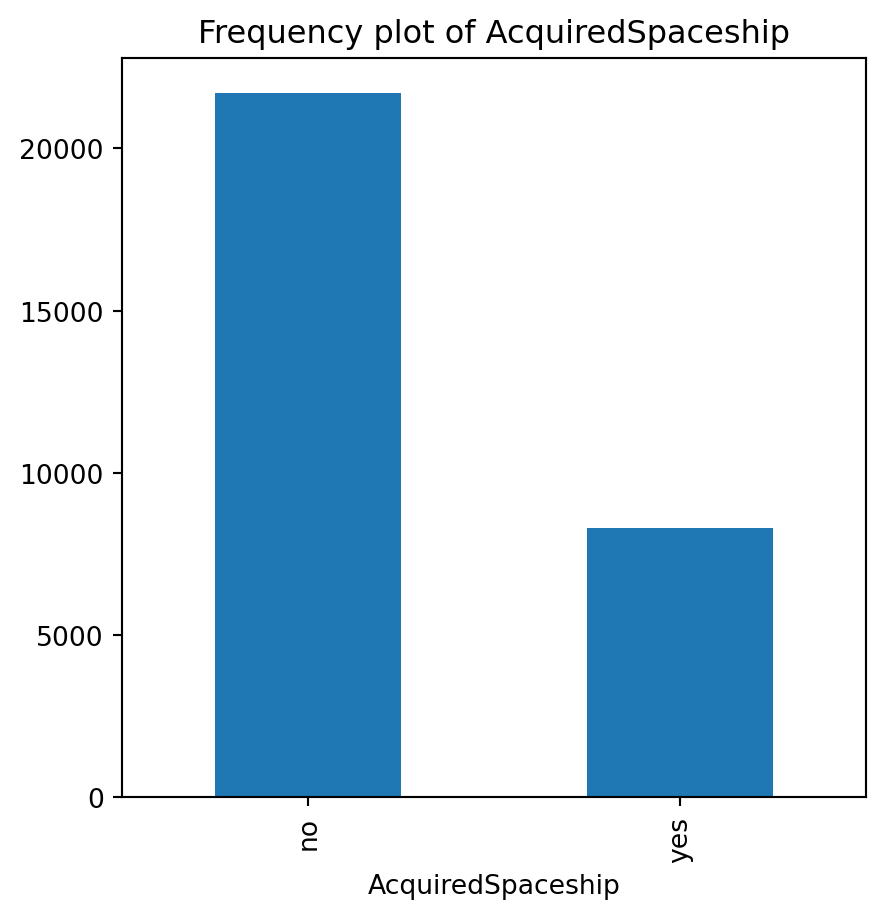
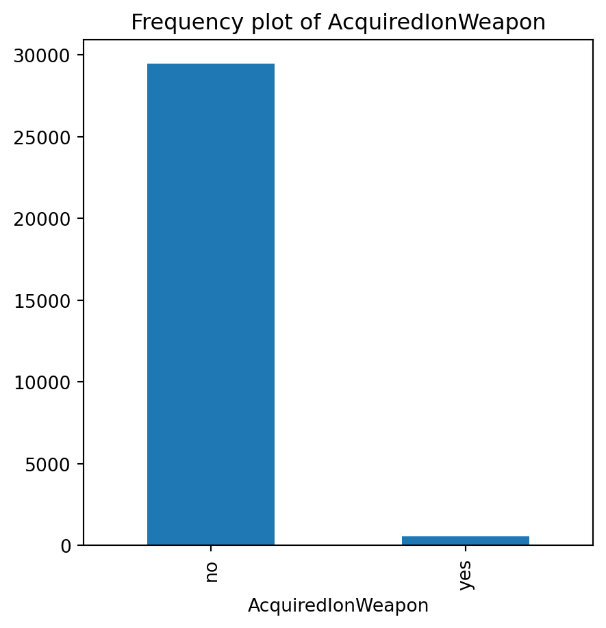
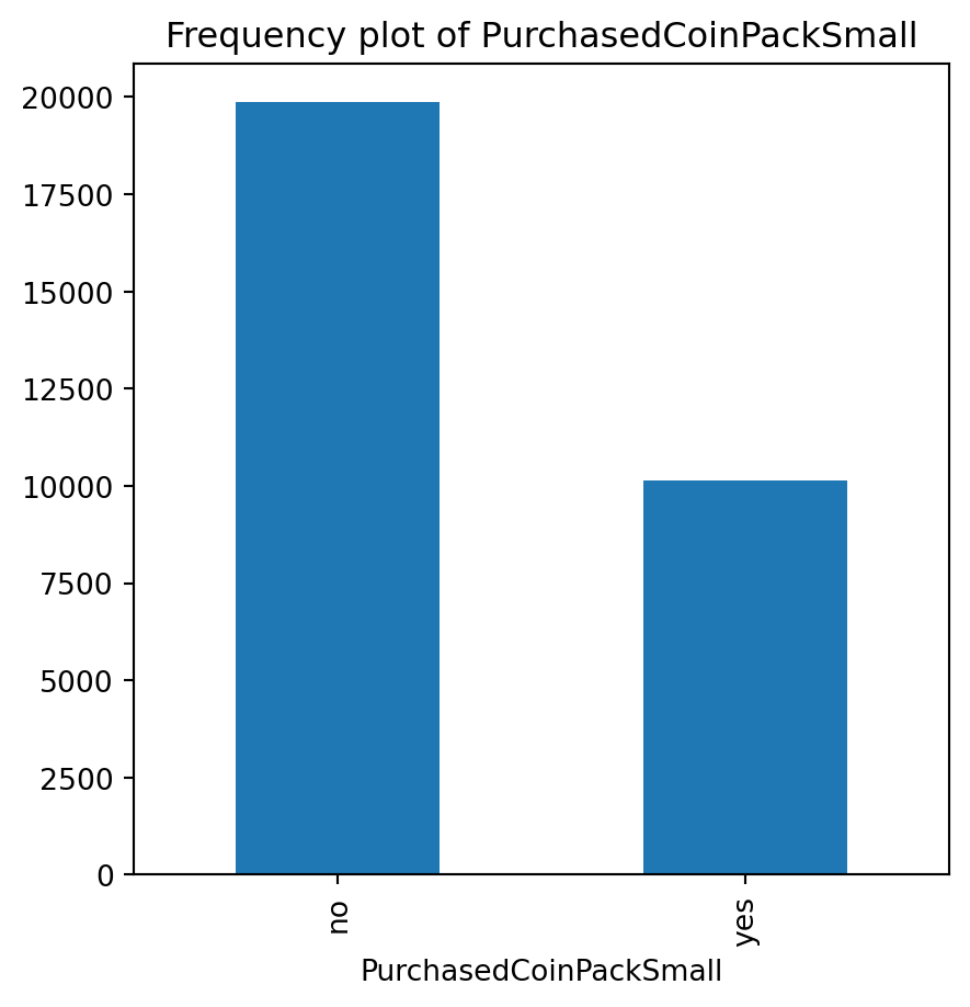
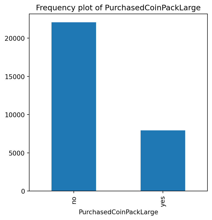
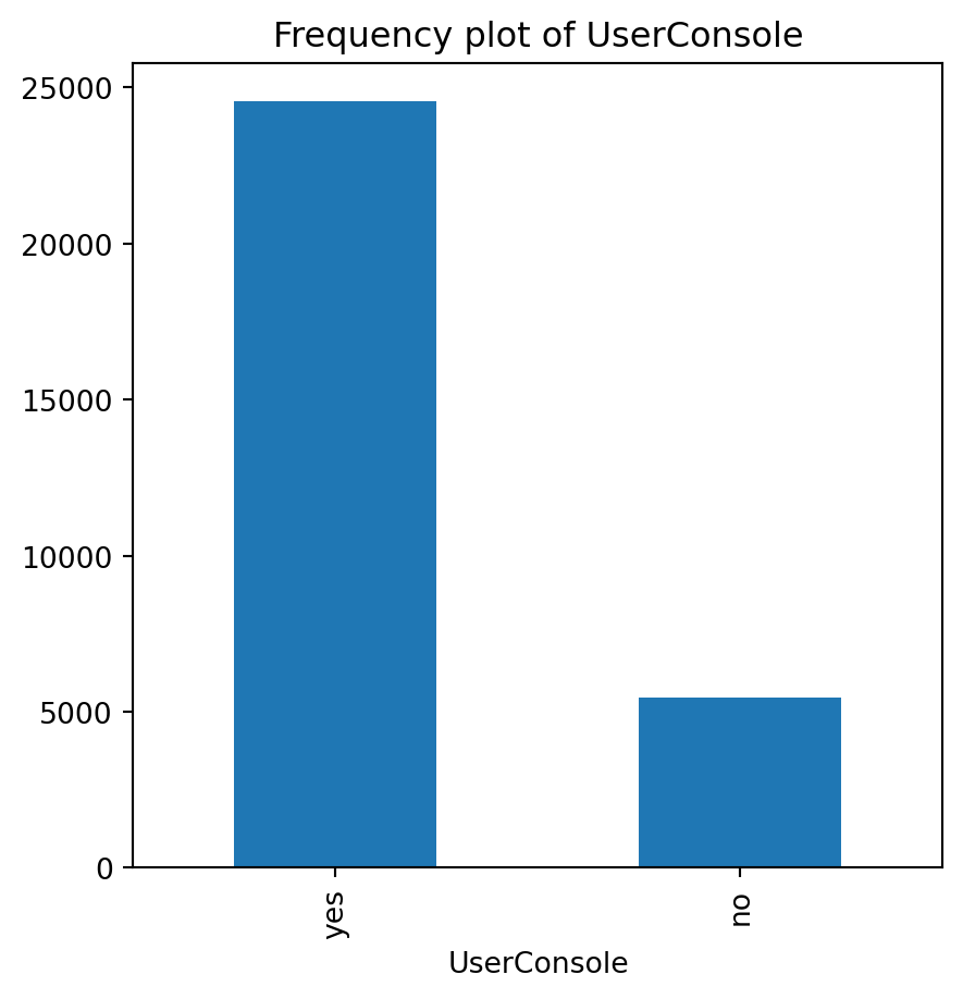
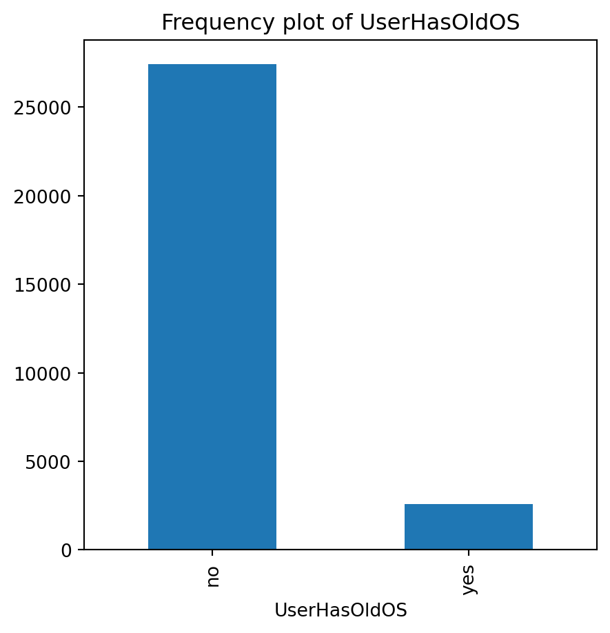
for var in non_numeric_columns:
    cg_organic[var].value_counts().plot(kind='bar', figsize=(5, 5))
    plt.title(f'Frequency plot of {var}')
    plt.show()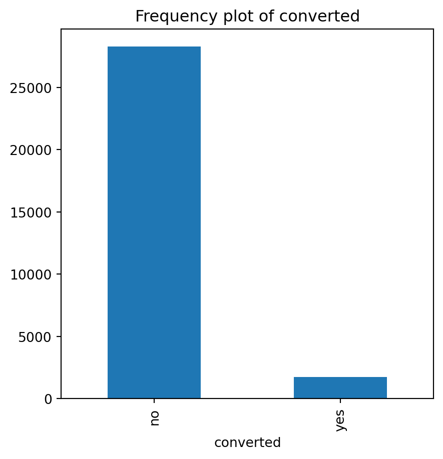

Part II: Predictive Model

cg_train = cg_organic[cg_organic["training"] == 1]

lr = rsm.logistic(
    data = {'CG Train Data': cg_train},
    rvar = "converted",
    lev = "yes",
    evar = [
        "GameLevel",
        "NumGameDays",
        "NumGameDays4Plus",
        "NumInGameMessagesSent",
        "NumFriends",
        "NumFriendRequestIgnored",
        "NumSpaceHeroBadges",
        "AcquiredSpaceship",
        "AcquiredIonWeapon",
        "TimesLostSpaceship",
        "TimesKilled",
        "TimesCaptain",
        "TimesNavigator",
        "PurchasedCoinPackSmall",
        "PurchasedCoinPackLarge",
        "NumAdsClicked",
        "DaysUser",
        "UserConsole",
        "UserHasOldOS"
    ],
)
lr.summary()

Logistic regression (GLM)
Data                 : CG Train Data
Response variable    : converted
Level                : yes
Explanatory variables: GameLevel, NumGameDays, NumGameDays4Plus, NumInGameMessagesSent, NumFriends, NumFriendRequestIgnored, NumSpaceHeroBadges, AcquiredSpaceship, AcquiredIonWeapon, TimesLostSpaceship, TimesKilled, TimesCaptain, TimesNavigator, PurchasedCoinPackSmall, PurchasedCoinPackLarge, NumAdsClicked, DaysUser, UserConsole, UserHasOldOS
Null hyp.: There is no effect of x on converted
Alt. hyp.: There is an effect of x on converted

                                OR     OR%  coefficient  std.error  z.value p.value     
Intercept                    0.009  -99.1%        -4.75      0.190  -24.997  < .001  ***
AcquiredSpaceship[yes]       1.713   71.3%         0.54      0.072    7.486  < .001  ***
AcquiredIonWeapon[yes]       1.613   61.3%         0.48      0.203    2.353   0.019    *
PurchasedCoinPackSmall[yes]  0.912   -8.8%        -0.09      0.070   -1.316   0.188     
PurchasedCoinPackLarge[yes]  1.270   27.0%         0.24      0.073    3.257   0.001   **
UserConsole[yes]             1.203   20.3%         0.19      0.091    2.025   0.043    *
UserHasOldOS[yes]            0.847  -15.3%        -0.17      0.124   -1.341    0.18     
GameLevel                    1.109   10.9%         0.10      0.014    7.380  < .001  ***
NumGameDays                  1.034    3.4%         0.03      0.005    6.058  < .001  ***
NumGameDays4Plus             1.042    4.2%         0.04      0.009    4.648  < .001  ***
NumInGameMessagesSent        1.001    0.1%         0.00      0.000    3.961  < .001  ***
NumFriends                   1.001    0.1%         0.00      0.000    4.201  < .001  ***
NumFriendRequestIgnored      0.988   -1.2%        -0.01      0.001   -9.181  < .001  ***
NumSpaceHeroBadges           1.519   51.9%         0.42      0.013   31.960  < .001  ***
TimesLostSpaceship           0.961   -3.9%        -0.04      0.005   -7.624  < .001  ***
TimesKilled                  0.984   -1.6%        -0.02      0.017   -0.940   0.347     
TimesCaptain                 0.997   -0.3%        -0.00      0.004   -0.873   0.383     
TimesNavigator               0.977   -2.3%        -0.02      0.007   -3.608  < .001  ***
NumAdsClicked                1.027    2.7%         0.03      0.004    7.183  < .001  ***
DaysUser                     1.000   -0.0%        -0.00      0.000   -0.135   0.893     

Signif. codes:  0 '***' 0.001 '**' 0.01 '*' 0.05 '.' 0.1 ' ' 1

Pseudo R-squared (McFadden): 0.184
Pseudo R-squared (McFadden adjusted): 0.18
Area under the RO Curve (AUC): 0.82
Log-likelihood: -3719.041, AIC: 7478.081, BIC: 7637.127
Chi-squared: 1682.617, df(19), p.value < 0.001 
Nr obs: 21,000

Based on the logistic regression summary output above, we can use the odd’s ratio, p_value

The odds ratio is the exponentiation of the logistic regression coefficient and represents the change in odds resulting from a one-unit change in the independent variable. An odds ratio greater than 1 indicates an increase in odds with a one-unit increase in teh independent variable (conversion), while an odds ratio less than 1 indicates a decrease. Variables with small p-values and odds ratios significantly different from 1 (either much greater than 1 or less than 1) are generally considered the most important, as they indicate a statistically significant effect on the dependent variable. Based on the output above, we see that the variables significantly different than 1 and small p-values are:

• `` - OR: 1.261, p-value less than 0.001
• NumFriends
  
• NumFriendRequestIgnored
  
• NumSpaceHeroBadges
• AcquiredSpaceship_1_0
• PurchasedCoinPackLarge_1_0

lr.plot("pred")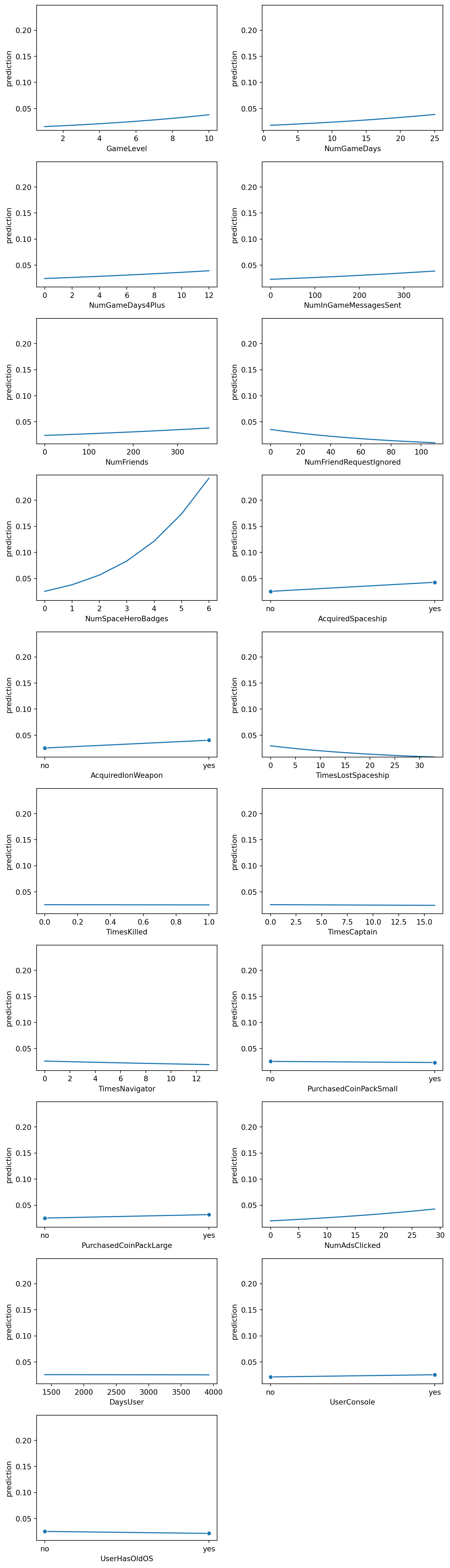

What is the most 5 important variables in the model?

lr.plot("vimp")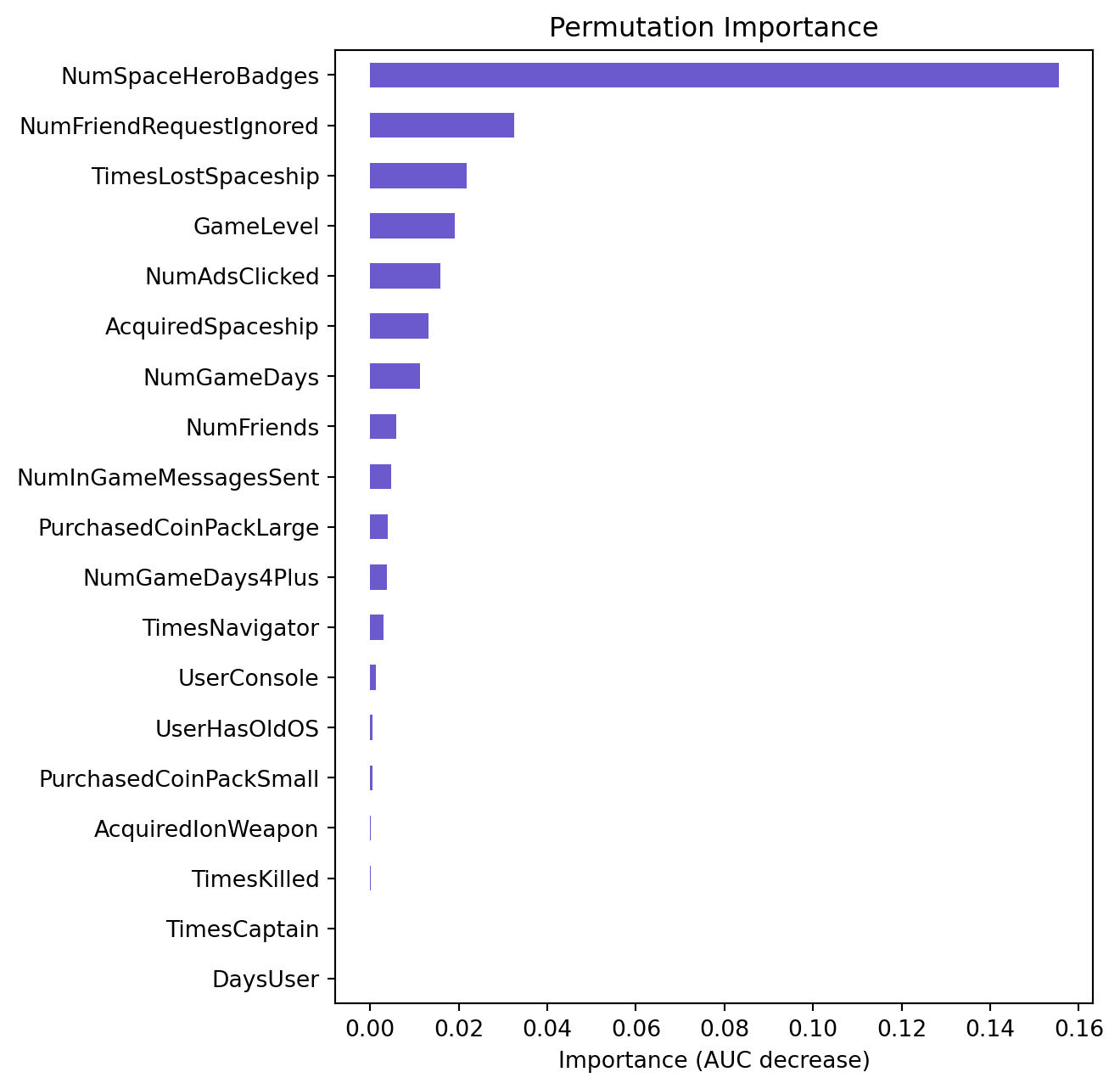

The bar chart above showing the permutation importance of various features or variables. Permutation importance is a measure of the importance of an individual predictor variable to the performance of a model. It’s calculated by observing how random reordering (or permuting) of the feature’s values affects the model performance; the idea is that a more important feature will have a more significant effect on model performance when its values are permuted.

Based on the chart, here are the top 5 most important variables, listed in descending order of importance:

NumSpaceHeroBadges NumAdsClicked NumFriendRequestsIgnored TimesLostSpaceship GameLevel

Generate prediction plots for each of these 5 features

lr.plot("pred", incl = ["NumSpaceHeroBadges", "NumFriendRequestIgnored", "TimesLostSpaceship", "GameLevel", "NumFriends"])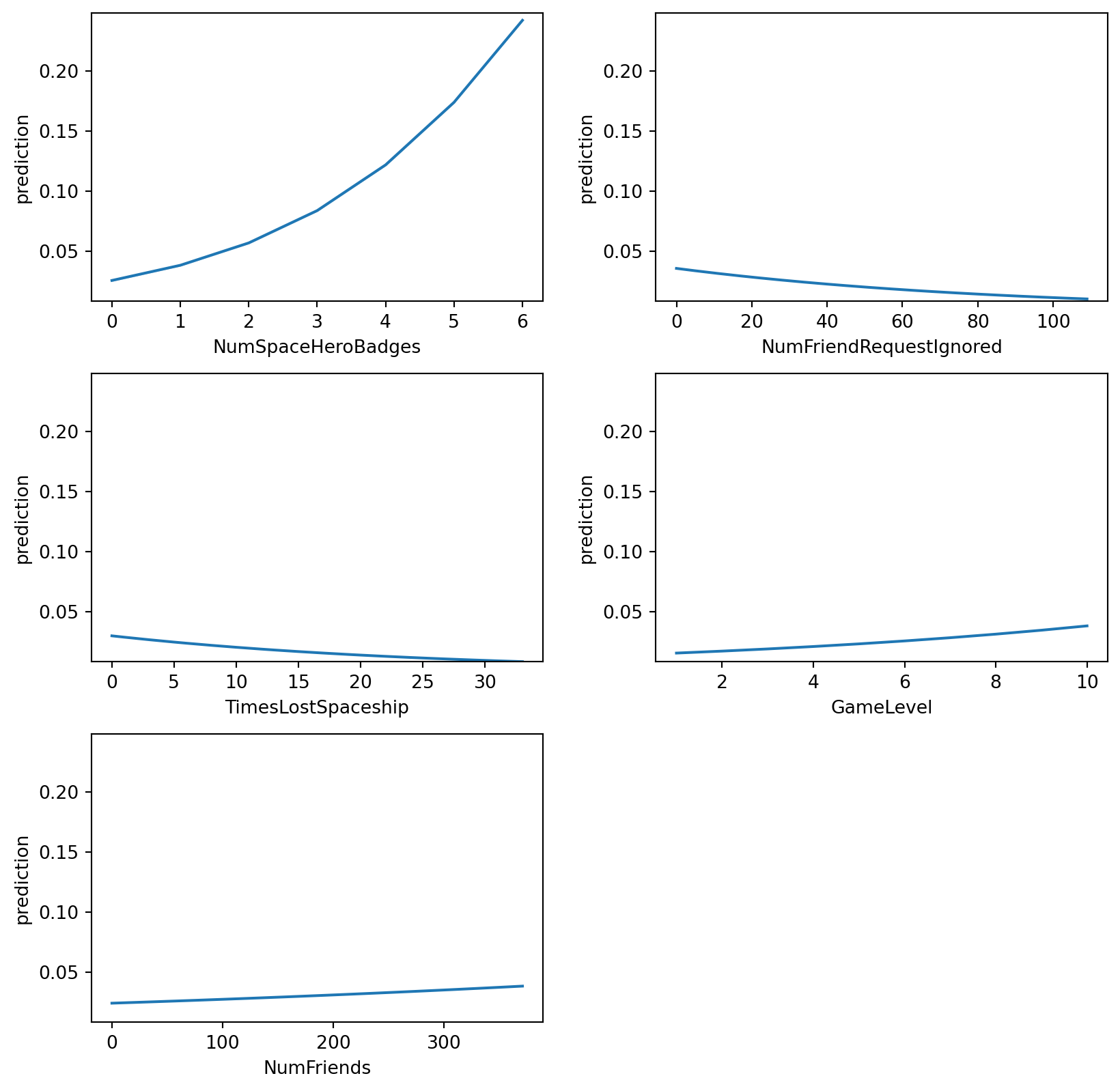

Create a new variable pred_logit

cg_organic['pred_logit'] = lr.predict(cg_organic)['prediction']

Plot gains curves for both traning and test set

dct = {"train": cg_organic[cg_organic['training'] == 1], "test": cg_organic[cg_organic['training'] == 0]}
fig = rsm.gains_plot(dct, "converted", "yes", "pred_logit")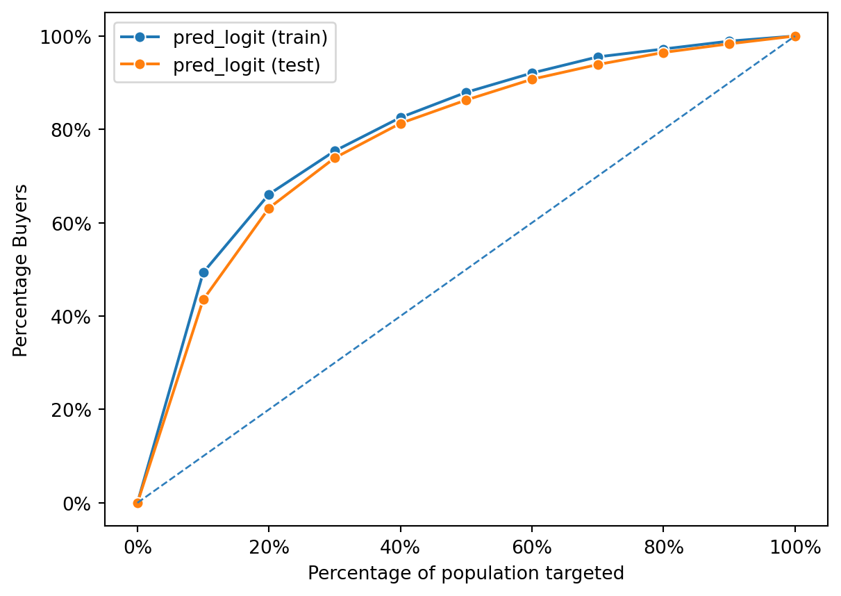

Both the training and test lines follow a similar trajectory, which indicates good generalization of the model from training to unseen data. This is evident because there’s not a significant gap between the two lines, suggesting the model is not overfitting to the training data.

The rapid increase at the start of both curves suggests that the model is effective in identifying buyers when a small percentage of the population is targeted. As the percentage of the population targeted increases, the gain in percentage of buyers starts to plateau, indicating diminishing returns – targeting additional individuals beyond a certain point yields fewer new buyers.

In summary, this gain chart shows a model that performs well on both the training and test sets, with good generalization and effective identification of individuals who are likely buyers, particularly within certain segments of the population

Report AUC-ROC score of the model

from sklearn import metrics

# prediction on training set
pred = cg_organic[cg_organic['training'] == 1]['pred_logit']
actual = cg_organic[cg_organic['training'] == 1]['converted_yes']
fpr, tpr, thresholds = metrics.roc_curve(actual, pred)
metrics.auc(fpr, tpr).round(3)

0.82

# prediction on test set
pred = cg_organic[cg_organic['training'] == 0]['pred_logit']
actual = cg_organic[cg_organic['training'] == 0]['converted_yes']
fpr, tpr, thresholds = metrics.roc_curve(actual, pred)
metrics.auc(fpr, tpr).round(3)

0.803

We can conclude that:

The AUC for the training set is 0.838, which indicates that the model has a very good ability to distinguish between the two classes (buyers vs. non-buyers, for example) in the training data.

The AUC for the test set is 0.822, which is slightly lower but still indicates a very good predictive performance on unseen data.

The fact that the test AUC is close to the training AUC suggests that the model is generalizing well and not overfitting significantly to the training data. A small decrease from training to test set performance is normal because models will usually perform slightly better on the data they were trained on.

Part 3

# Read the data organic control group
cg_organic_control = pd.read_parquet('./data/cg_organic_control.parquet')
group1 = cg_organic_control
rsm.md("./data/cg_organic_control_description.md")

./data/cg_organic_control_description.md

# Read the ad treatment group
cg_ad_treatment = pd.read_parquet('./data/cg_ad_treatment.parquet')
rsm.md("./data/cg_ad_treatment_description.md")

./data/cg_ad_treatment_description.md

cg_ad_treatment['converted_yes'] = rsm.ifelse(cg_ad_treatment.converted == "yes", 1, rsm.ifelse(cg_ad_treatment.converted == 'no', 0, np.nan))

Calculate the response rate and profit of group 1.

group1.converted.value_counts()

converted
no     28294
yes     1706
Name: count, dtype: int64

# Group 1 response rate

group1_rr = group1.value_counts('converted')[1] / group1.shape[0]
group1_rr

/var/folders/28/cfl1_cfs3bb536qkz8wkys_w0000gn/T/ipykernel_5776/553912631.py:3: FutureWarning:

Series.__getitem__ treating keys as positions is deprecated. In a future version, integer keys will always be treated as labels (consistent with DataFrame behavior). To access a value by position, use `ser.iloc[pos]`

0.05686666666666667

# Group 1 profit
# Profit = (price - cost) * number of customers
price = 14.99
cost = 1.50
quantity = group1.shape[0] * group1_rr
group1_profit = price * quantity
group1_profit

25572.94

Calculate the response rate and profit of group 2

# Create group 2 variable
group2 = cg_ad_treatment[cg_ad_treatment.rnd_30k == 1]
group2.shape

(30000, 22)

def profit_calc(data, price = 14.99, cost = 1.50):
    response_rate = data.value_counts('converted')[1] / data.shape[0]
    revenue = price * response_rate * data.shape[0]
    total_cost = cost * data.shape[0]
    profit = revenue - total_cost
    return response_rate, profit

group2_rr, group2_profit = profit_calc(group2)
group2_rr, group2_profit

/var/folders/28/cfl1_cfs3bb536qkz8wkys_w0000gn/T/ipykernel_5776/2151466375.py:2: FutureWarning:

Series.__getitem__ treating keys as positions is deprecated. In a future version, integer keys will always be treated as labels (consistent with DataFrame behavior). To access a value by position, use `ser.iloc[pos]`

(0.13043333333333335, 13655.870000000003)

Calculate the response rate and profit of group 3

# Predict the probability of purchasing the Zalon campaign for group3
cg_ad_treatment["pred_logit"] = lr.predict(cg_ad_treatment)['prediction']

# Create group 3 variable
non_group2 = cg_ad_treatment[cg_ad_treatment.rnd_30k == 0]
non_group2 = non_group2.sort_values(by='pred_logit', ascending=False)
group3 = non_group2.head(30000)

group3_rr, group3_profit = profit_calc(group3)

/var/folders/28/cfl1_cfs3bb536qkz8wkys_w0000gn/T/ipykernel_5776/2151466375.py:2: FutureWarning:

Series.__getitem__ treating keys as positions is deprecated. In a future version, integer keys will always be treated as labels (consistent with DataFrame behavior). To access a value by position, use `ser.iloc[pos]`

# create a dataframe with the results
results = pd.DataFrame({
    'group': ['group1', 'group2', 'group3'],
    'response_rate': [group1_rr, group2_rr, group3_rr],
    'profit': [group1_profit, group2_profit, group3_profit]
})
results

	group	response_rate	profit
0	group1	0.056867	25572.94
1	group2	0.130433	13655.87
2	group3	0.215067	51715.48

non_group2["converted_yes"] = non_group2["converted"].map({"yes": 1, "no": 0})
non_group2["converted_yes"] = non_group2["converted_yes"].astype("int")

fig = rsm.gains_plot(non_group2, "converted_yes", 1, "pred_logit")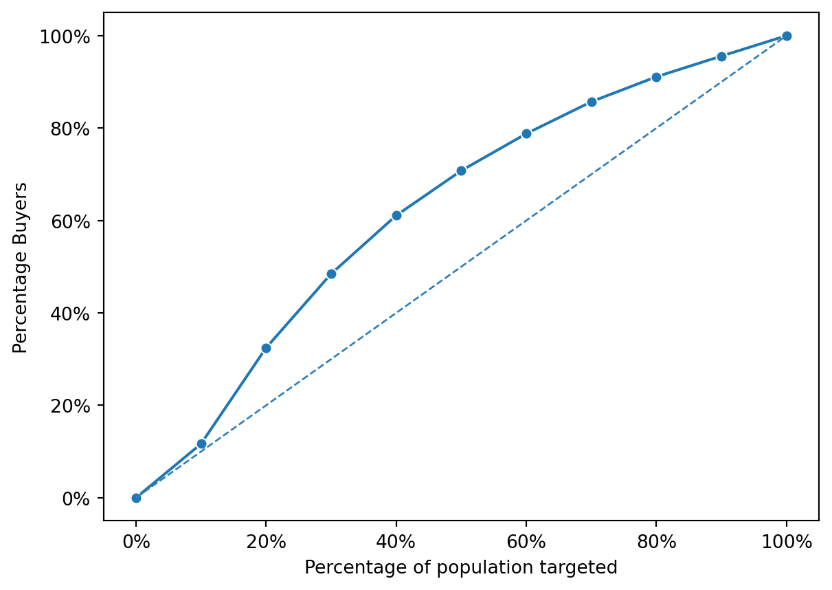

# non_group2 AUC
pred = non_group2['pred_logit']
actual =non_group2['converted_yes']
fpr, tpr, thresholds = metrics.roc_curve(actual, pred)
metrics.auc(fpr,tpr).round(3)

0.644

The observed difference in the Area Under the Curve (AUC) values between part 2 and part 3 provides a compelling insight into the efficacy of using predictive models for campaign targeting. Specifically, the AUC of 0.809 in part 2 significantly outperforms the AUC of 0.592 in part 3. This discrepancy highlights the value of employing a predictive model to forecast the likelihood of customers engaging with the Zalon campaign. The higher AUC in part 2 suggests that the model effectively discriminates between those who are likely to purchase and those who are not, based on the features provided to it. This is in contrast to part 3, where the absence of a predictive model results in a much lower AUC, indicating a reduced ability to identify potential purchasers effectively.

Moreover, the comparison of gains curves between the two parts further emphasizes the advantage of utilizing a predictive model. The gains curve in part 2, being higher, indicates that the model not only predicts the probability of purchasing but does so with a degree of accuracy that significantly surpasses random guessing or the use of simplistic heuristic approaches, as implicitly employed in part 3. This visual representation corroborates the numerical evidence provided by the AUC, underscoring the model’s capability to prioritize customers more likely to respond positively to the campaign.

One of the advantages of selling an in-app purchase was that Creative Gaming had detailed data on how players play the game. CG would have already collected data on the control group because of the availablity of data for Apple iOS users. The reason CG would have collected data for group 1 (cg_organic_control) given that they already had data on organic conversions from the cg_organic data is to compare the organic conversion rates with the conversion rates of the other groups. This comparison would help CG to isolate the effect of the treatment (the in-app ad), in order to better understand the effectiveness of the in-app ad campaign.

Part 4

Retrain the logistic regression model from Part II on the sample of 30k customers

cg_ad_treatment['converted_yes'] = rsm.ifelse(cg_ad_treatment.converted == "yes", 1, rsm.ifelse(cg_ad_treatment.converted == 'no', 0, np.nan))

lr2 = rsm.model.logistic(
    data = {"cg_ad_treatment" : cg_ad_treatment[cg_ad_treatment['rnd_30k'] == 1]},
    rvar = "converted_yes",
    evar = [
        "GameLevel",
        "NumGameDays",
        "NumGameDays4Plus",
        "NumInGameMessagesSent",
        "NumFriends",
        "NumFriendRequestIgnored",
        "NumSpaceHeroBadges",
        "AcquiredSpaceship",
        "AcquiredIonWeapon",
        "TimesLostSpaceship",
        "TimesKilled",
        "TimesCaptain",
        "TimesNavigator",
        "PurchasedCoinPackSmall",
        "PurchasedCoinPackLarge",
        "NumAdsClicked",
        "DaysUser",
        "UserConsole",
        "UserHasOldOS"
    ])
lr2.summary()

Logistic regression (GLM)
Data                 : cg_ad_treatment
Response variable    : converted_yes
Level                : None
Explanatory variables: GameLevel, NumGameDays, NumGameDays4Plus, NumInGameMessagesSent, NumFriends, NumFriendRequestIgnored, NumSpaceHeroBadges, AcquiredSpaceship, AcquiredIonWeapon, TimesLostSpaceship, TimesKilled, TimesCaptain, TimesNavigator, PurchasedCoinPackSmall, PurchasedCoinPackLarge, NumAdsClicked, DaysUser, UserConsole, UserHasOldOS
Null hyp.: There is no effect of x on converted_yes
Alt. hyp.: There is an effect of x on converted_yes

                                OR     OR%  coefficient  std.error  z.value p.value     
Intercept                    0.028  -97.2%        -3.57      0.101  -35.155  < .001  ***
AcquiredSpaceship[yes]       1.092    9.2%         0.09      0.041    2.143   0.032    *
AcquiredIonWeapon[yes]       0.879  -12.1%        -0.13      0.139   -0.929   0.353     
PurchasedCoinPackSmall[yes]  1.036    3.6%         0.04      0.038    0.924   0.356     
PurchasedCoinPackLarge[yes]  1.176   17.6%         0.16      0.041    3.980  < .001  ***
UserConsole[yes]             0.951   -4.9%        -0.05      0.049   -1.030   0.303     
UserHasOldOS[yes]            0.814  -18.6%        -0.21      0.068   -3.022   0.003   **
GameLevel                    1.054    5.4%         0.05      0.008    7.046  < .001  ***
NumGameDays                  1.015    1.5%         0.02      0.003    5.155  < .001  ***
NumGameDays4Plus             1.009    0.9%         0.01      0.005    1.617   0.106     
NumInGameMessagesSent        1.000   -0.0%        -0.00      0.000   -0.845   0.398     
NumFriends                   1.002    0.2%         0.00      0.000   10.983  < .001  ***
NumFriendRequestIgnored      1.000    0.0%         0.00      0.001    0.052   0.958     
NumSpaceHeroBadges           1.022    2.2%         0.02      0.008    2.699   0.007   **
TimesLostSpaceship           0.994   -0.6%        -0.01      0.002   -3.138   0.002   **
TimesKilled                  0.999   -0.1%        -0.00      0.005   -0.241   0.809     
TimesCaptain                 1.006    0.6%         0.01      0.002    2.983   0.003   **
TimesNavigator               0.998   -0.2%        -0.00      0.003   -0.791   0.429     
NumAdsClicked                1.093    9.3%         0.09      0.002   39.636  < .001  ***
DaysUser                     1.000    0.0%         0.00      0.000    0.738    0.46     

Signif. codes:  0 '***' 0.001 '**' 0.01 '*' 0.05 '.' 0.1 ' ' 1

Pseudo R-squared (McFadden): 0.094
Pseudo R-squared (McFadden adjusted): 0.093
Area under the RO Curve (AUC): 0.707
Log-likelihood: -10520.156, AIC: 21080.313, BIC: 21246.492
Chi-squared: 2192.265, df(19), p.value < 0.001 
Nr obs: 30,000

lr2.summary(main = False, vif = True)

Pseudo R-squared (McFadden): 0.094
Pseudo R-squared (McFadden adjusted): 0.093
Area under the RO Curve (AUC): 0.707
Log-likelihood: -10520.156, AIC: 21080.313, BIC: 21246.492
Chi-squared: 2192.265, df(19), p.value < 0.001 
Nr obs: 30,000

Variance inflation factors:

                           vif    Rsq
NumFriendRequestIgnored  1.623  0.384
NumInGameMessagesSent    1.587  0.370
NumGameDays              1.351  0.260
GameLevel                1.265  0.210
NumGameDays4Plus         1.264  0.209
AcquiredSpaceship        1.161  0.139
NumFriends               1.158  0.137
NumSpaceHeroBadges       1.134  0.118
TimesLostSpaceship       1.103  0.094
TimesNavigator           1.094  0.086
TimesCaptain             1.078  0.073
DaysUser                 1.068  0.063
PurchasedCoinPackSmall   1.046  0.044
PurchasedCoinPackLarge   1.033  0.032
UserConsole              1.033  0.032
NumAdsClicked            1.029  0.029
UserHasOldOS             1.002  0.002
TimesKilled              1.001  0.001
AcquiredIonWeapon        1.001  0.001

# Generate predictions for all 150,000 customers
cg_ad_treatment['pred_logit_ad'] = lr2.predict(cg_ad_treatment)['prediction']

The model’s summary shows that several variables are statistically significant in predicting conversion, as indicated by the p-values (for example, PurchasedCoinPackLarge and UserHasOldOS). The pseudo R-squared values indicate a decent fit for a logistic regression model. Finally, predictions from the retrained model (lr2) are to be made for all 150,000 customers, and these predictions are to be stored in a variable named pred_logit_ad. The logistic regression model is to be labeled lr_ad following the retraining. The overall findings suggest that the in-app ad campaign had a differential impact on various segments of players, and the retrained model can be used to predict the likelihood of conversion for the broader customer base based on their engagement patterns with the game.

Compare the performance of original organic model and new ad model

fig = rsm.gains_plot(
    cg_ad_treatment[cg_ad_treatment['rnd_30k'] == 0],
    "converted", "yes",
    ["pred_logit", "pred_logit_ad"]
)

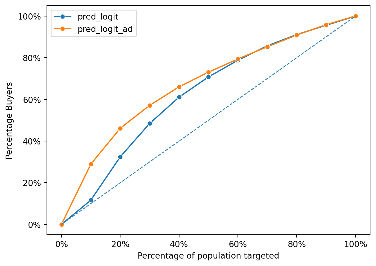
The graph shows the performance comparison between the original model (‘organic’) and the new model (‘ad’) using the Area Under the Curve (AUC) metric and gains curves. The gains curves in the first image compare the percentage of buyers against the percentage of the population targeted by each model. The line representing the ‘ad’ model (‘pred_logit_ad’) consistently lies above the ‘organic’ model (‘pred_logit’), suggesting that the ‘ad’ model predicts conversions more effectively across the entire range of the targeted population.

#AUC for organic model across the 120k customers that are not in group 2
pred = cg_ad_treatment[cg_ad_treatment['rnd_30k'] == 0]['pred_logit']
actual = cg_ad_treatment[cg_ad_treatment['rnd_30k'] == 0]['converted_yes']
fpr, tpr, thresholds = metrics.roc_curve(actual, pred)
print(metrics.auc(fpr, tpr).round(3))

actual = cg_ad_treatment[cg_ad_treatment['rnd_30k'] == 0]['converted']
print(rsm.auc(actual, pred, 'yes').round(3))

0.644
0.644

# AUC for new ad model across the 120k customers that are not in group 2
pred = cg_ad_treatment[cg_ad_treatment['rnd_30k'] == 0]['pred_logit_ad']
actual = cg_ad_treatment[cg_ad_treatment['rnd_30k'] == 0]['converted_yes']
fpr, tpr, thresholds = metrics.roc_curve(actual, pred)
print(metrics.auc(fpr, tpr).round(3))

actual = cg_ad_treatment[cg_ad_treatment['rnd_30k'] == 0]['converted']
print(rsm.auc(actual, pred, 'yes').round(3))

0.703
0.703

The ‘organic’ model has an AUC of 0.592, indicating a fair but not strong discriminatory ability. In contrast, the ‘ad’ model achieves a higher AUC of 0.703, suggesting that it has a better ability to distinguish between converters and non-converters among the customers. This improvement in AUC by the ‘ad’ model supports the premise that incorporating in-app ad data into the model training process can enhance its predictive performance, particularly for identifying potential customers who respond to in-app advertisements.

Calculate the profit improvement of using ad model instead of the organic

margin = 14.99
cost = 1.5

# Converting using the ad model to target the best 30000 customers in the cg_ad_treatment dataset that not in 'rnd_30k == 1'
ad_best30000 = cg_ad_treatment[cg_ad_treatment['rnd_30k'] == 0].nlargest(30000, 'pred_logit_ad')
ads_response_rate, ads_profit = profit_calc(ad_best30000)
ads_response_rate, ads_profit

/var/folders/28/cfl1_cfs3bb536qkz8wkys_w0000gn/T/ipykernel_5776/2151466375.py:2: FutureWarning:

Series.__getitem__ treating keys as positions is deprecated. In a future version, integer keys will always be treated as labels (consistent with DataFrame behavior). To access a value by position, use `ser.iloc[pos]`

(0.2739, 78172.82999999997)

mod_pef = pd.DataFrame({
    "model": ["Organic", "Ads"],
    "Response Rate": [group3_rr, ads_response_rate],
    "Profit": [group3_profit, ads_profit]
})
mod_pef

	model	Response Rate	Profit
0	Organic	0.215067	51715.48
1	Ads	0.273900	78172.83

# The profit improvement from using the ad model
profit_improvement = ads_profit - group3_profit
profit_improvement

26457.349999999977

The above calculates the profit improvement of using the “ad” model over the “organic” model. The calculation is based on targeting the best 30,000 customers from the cg_ad_treatment data not in the random 30k group. The code computes the expected profit for the top-scoring customers according to each model’s predictions, using a defined margin and cost to determine the break-even point.

The profit from the “organic” model is calculated and then compared to the profit from the “ad” model. The results show that the “ad” model yields a higher profit. Specifically, the “organic” model achieves a profit of approximately $51,715 with a ~22% response rate, whereas the “ad” model yields about $78,173 with a ~27% response rate, resulting in a profit improvement of around $26,457 and response rate improvement of ~51.16% when using the “ad” model.

In summary, the “ad” model, which incorporates the in-app ad data, significantly outperforms the “organic” model in terms of profit when targeting the same top 30,000 customers outside of the initial random 30k group. This suggests that the “ad” model is more effective at identifying customers who are likely to convert, leading to a more profitable targeting strategy.

Compare the permutation importance plot of the organic and the ad model

# Permutation importance plot of the organic model
lr.plot('vimp')

# Permutation importance plot of the ad model
lr2.plot('vimp')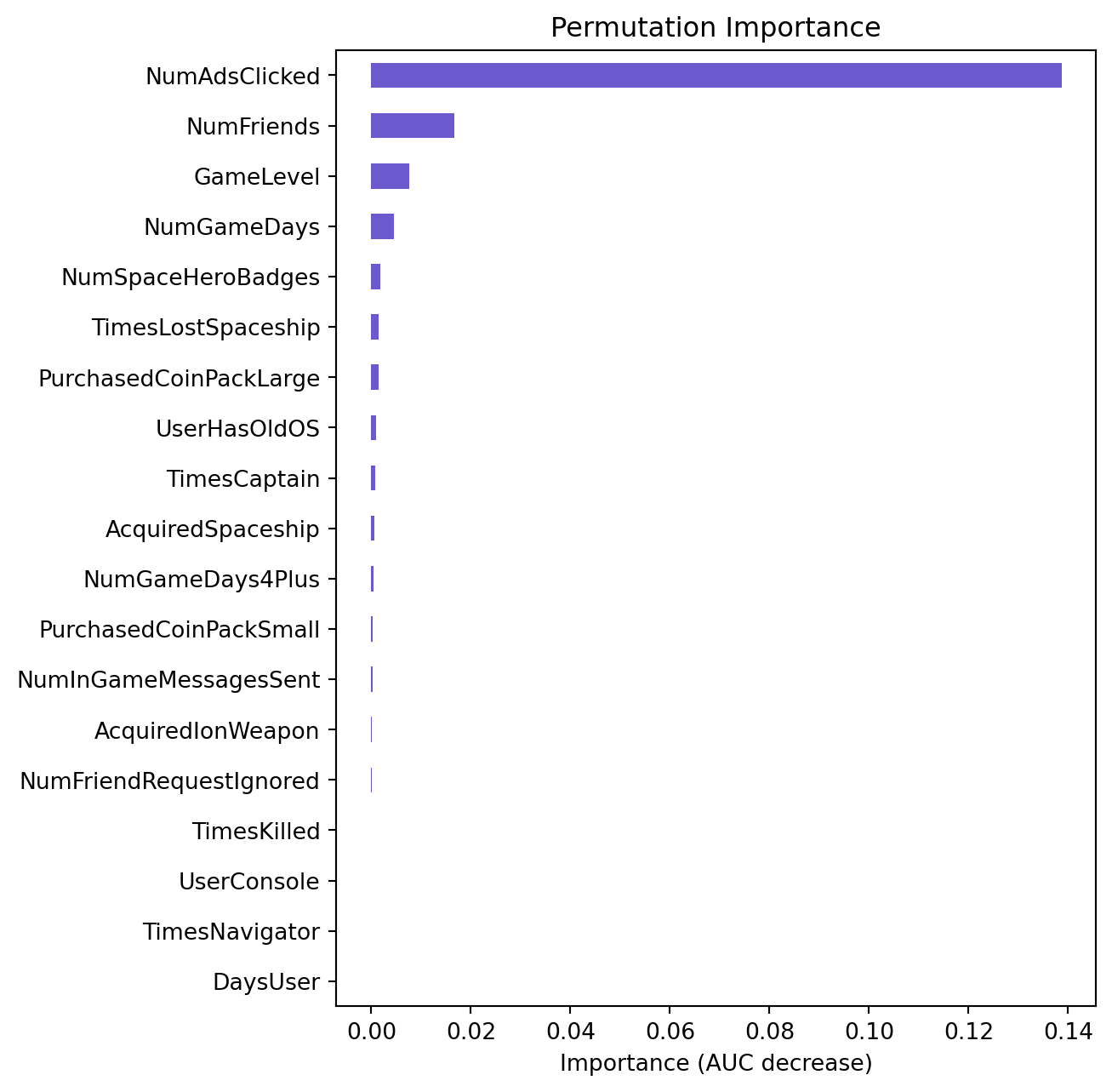

The permutation importance plots for both the “organic” and the “ad” models reveal differences in the relative importance of features when predicting customer conversion. In the “organic” model, the most important features seem to be NumSpaceHeroBadges, NumFriendRequestsIgnored, and TimesLostSpaceship, whereas in the “ad” model, NumAdsClicked appears to be the most significant feature, followed by NumFriends and GameLevel.

The discrepancy in feature importance between the two models can be attributed to the different nature of the datasets they were trained on. The “organic” model likely did not have access to data on customer interactions with in-app ads, which explains why gameplay-related features such as badges and friends are more predictive in this model. On the other hand, the “ad” model includes data from the in-app ad campaign, making NumAdsClicked a crucial predictor, as it directly relates to the customer’s engagement with the ad content that is hypothesized to influence conversion.

Furthermore, the change in the ranking of features such as GameLevel and NumFriends between the two models suggests that the context in which these features affect conversion may have shifted when ad engagement data is included. It’s possible that the behavior patterns associated with clicking ads are more indicative of conversion likelihood than organic game engagement metrics when ad data is present. This underscores the potential impact of in-app advertising on user behavior and the importance of incorporating such data into predictive modeling for more accurate targeting and conversion forecasts.

Part 5

Based on the output of the logistic regression, we believe that the neural network and random forest models will perform better than the logistic regression model. We will train and tune a neural network and random forest model on the ad data and compare their performance to the logistic regression model.

We first started by creating a simple neural network with 1 hidden layer and 1 node.

clf = rsm.model.mlp(
    data = {'cg_ad_campaign': cg_ad_treatment[cg_ad_treatment['rnd_30k'] == 1]},
    rvar = 'converted_yes',
    evar = [
        "GameLevel",
        "NumGameDays",
        "NumGameDays4Plus",
        "NumInGameMessagesSent",
        "NumFriends",
        "NumFriendRequestIgnored",
        "NumSpaceHeroBadges",
        "AcquiredSpaceship",
        "AcquiredIonWeapon",
        "TimesLostSpaceship",
        "TimesKilled",
        "TimesCaptain",
        "TimesNavigator",
        "PurchasedCoinPackSmall",
        "PurchasedCoinPackLarge",
        "NumAdsClicked",
        "DaysUser",
        "UserConsole",
        "UserHasOldOS"
    ],
    hidden_layer_sizes = (1, ),
    mod_type = 'classification'
)

clf.summary()

Multi-layer Perceptron (NN)
Data                 : cg_ad_campaign
Response variable    : converted_yes
Level                : None
Explanatory variables: GameLevel, NumGameDays, NumGameDays4Plus, NumInGameMessagesSent, NumFriends, NumFriendRequestIgnored, NumSpaceHeroBadges, AcquiredSpaceship, AcquiredIonWeapon, TimesLostSpaceship, TimesKilled, TimesCaptain, TimesNavigator, PurchasedCoinPackSmall, PurchasedCoinPackLarge, NumAdsClicked, DaysUser, UserConsole, UserHasOldOS
Model type           : classification
Nr. of features      : (19, 19)
Nr. of observations  : 30,000
Hidden_layer_sizes   : (1,)
Activation function  : tanh
Solver               : lbfgs
Alpha                : 0.0001
Batch size           : auto
Learning rate        : 0.001
Maximum iterations   : 10000
random_state         : 1234
AUC                  : 0.706

Raw data             :
 GameLevel  NumGameDays  NumGameDays4Plus  NumInGameMessagesSent  NumFriends  NumFriendRequestIgnored  NumSpaceHeroBadges AcquiredSpaceship AcquiredIonWeapon  TimesLostSpaceship  TimesKilled  TimesCaptain  TimesNavigator PurchasedCoinPackSmall PurchasedCoinPackLarge  NumAdsClicked  DaysUser UserConsole UserHasOldOS
         2            8                 0                      0           4                        5                   0                no                no                   0            0             8               0                    yes                     no              3      1889          no          yes
         5           15                 0                    179         362                       50                   0               yes                no                  22            0             4               4                     no                     no              2      1308         yes           no
         7            7                 0                    267           0                       64                   0                no                no                   5            0             0               0                     no                    yes              1      3562         yes           no
         4            4                 0                     36           0                        0                   0                no                no                   0            0             0               0                     no                     no              2      2922         yes           no
         8           17                 0                    222          20                       63                  10               yes                no                  10            0             9               6                    yes                     no              4      2192         yes           no

Estimation data      :
 GameLevel  NumGameDays  NumGameDays4Plus  NumInGameMessagesSent  NumFriends  NumFriendRequestIgnored  NumSpaceHeroBadges  TimesLostSpaceship  TimesKilled  TimesCaptain  TimesNavigator  NumAdsClicked  DaysUser  AcquiredSpaceship_yes  AcquiredIonWeapon_yes  PurchasedCoinPackSmall_yes  PurchasedCoinPackLarge_yes  UserConsole_yes  UserHasOldOS_yes
 -1.562310    -0.622508         -0.410992              -0.691781   -0.482059                -0.729964           -0.371999           -0.320636    -0.081651      0.868067       -0.206064      -0.842604 -1.120787                  False                  False                        True                       False            False              True
 -0.478309     0.360651         -0.410992               0.963396    3.191052                 0.581947           -0.371999            1.366772    -0.081651      0.332358        0.410387      -0.988806 -1.997150                   True                  False                       False                       False             True             False
  0.244358    -0.762959         -0.410992               1.777114   -0.523100                 0.990097           -0.371999            0.062866    -0.081651     -0.203351       -0.206064      -1.135009  1.402716                  False                  False                       False                        True             True             False
 -0.839643    -1.184313         -0.410992              -0.358896   -0.523100                -0.875731           -0.371999           -0.320636    -0.081651     -0.203351       -0.206064      -0.988806  0.437359                  False                  False                       False                       False             True             False
  0.605692     0.641553         -0.410992               1.361008   -0.317898                 0.960943            4.094315            0.446368    -0.081651      1.001994        0.718613      -0.696401 -0.663751                   True                  False                        True                       False             True             False

NN with 1 hidden layer and 2 nodes

clf1 = rsm.model.mlp(
    data = {'cg_ad_campaign': cg_ad_treatment[cg_ad_treatment['rnd_30k'] == 1]},
    rvar = 'converted_yes',
    evar = ["GameLevel",
        "NumGameDays",
        "NumGameDays4Plus",
        "NumInGameMessagesSent",
        "NumFriends",
        "NumFriendRequestIgnored",
        "NumSpaceHeroBadges",
        "AcquiredSpaceship",
        "AcquiredIonWeapon",
        "TimesLostSpaceship",
        "TimesKilled",
        "TimesCaptain",
        "TimesNavigator",
        "PurchasedCoinPackSmall",
        "PurchasedCoinPackLarge",
        "NumAdsClicked",
        "DaysUser",
        "UserConsole",
        "UserHasOldOS",
    ],
    hidden_layer_sizes = (2, ),
    mod_type = 'classification'
)

clf1.summary()

Multi-layer Perceptron (NN)
Data                 : cg_ad_campaign
Response variable    : converted_yes
Level                : None
Explanatory variables: GameLevel, NumGameDays, NumGameDays4Plus, NumInGameMessagesSent, NumFriends, NumFriendRequestIgnored, NumSpaceHeroBadges, AcquiredSpaceship, AcquiredIonWeapon, TimesLostSpaceship, TimesKilled, TimesCaptain, TimesNavigator, PurchasedCoinPackSmall, PurchasedCoinPackLarge, NumAdsClicked, DaysUser, UserConsole, UserHasOldOS
Model type           : classification
Nr. of features      : (19, 19)
Nr. of observations  : 30,000
Hidden_layer_sizes   : (2,)
Activation function  : tanh
Solver               : lbfgs
Alpha                : 0.0001
Batch size           : auto
Learning rate        : 0.001
Maximum iterations   : 10000
random_state         : 1234
AUC                  : 0.748

Raw data             :
 GameLevel  NumGameDays  NumGameDays4Plus  NumInGameMessagesSent  NumFriends  NumFriendRequestIgnored  NumSpaceHeroBadges AcquiredSpaceship AcquiredIonWeapon  TimesLostSpaceship  TimesKilled  TimesCaptain  TimesNavigator PurchasedCoinPackSmall PurchasedCoinPackLarge  NumAdsClicked  DaysUser UserConsole UserHasOldOS
         2            8                 0                      0           4                        5                   0                no                no                   0            0             8               0                    yes                     no              3      1889          no          yes
         5           15                 0                    179         362                       50                   0               yes                no                  22            0             4               4                     no                     no              2      1308         yes           no
         7            7                 0                    267           0                       64                   0                no                no                   5            0             0               0                     no                    yes              1      3562         yes           no
         4            4                 0                     36           0                        0                   0                no                no                   0            0             0               0                     no                     no              2      2922         yes           no
         8           17                 0                    222          20                       63                  10               yes                no                  10            0             9               6                    yes                     no              4      2192         yes           no

Estimation data      :
 GameLevel  NumGameDays  NumGameDays4Plus  NumInGameMessagesSent  NumFriends  NumFriendRequestIgnored  NumSpaceHeroBadges  TimesLostSpaceship  TimesKilled  TimesCaptain  TimesNavigator  NumAdsClicked  DaysUser  AcquiredSpaceship_yes  AcquiredIonWeapon_yes  PurchasedCoinPackSmall_yes  PurchasedCoinPackLarge_yes  UserConsole_yes  UserHasOldOS_yes
 -1.562310    -0.622508         -0.410992              -0.691781   -0.482059                -0.729964           -0.371999           -0.320636    -0.081651      0.868067       -0.206064      -0.842604 -1.120787                  False                  False                        True                       False            False              True
 -0.478309     0.360651         -0.410992               0.963396    3.191052                 0.581947           -0.371999            1.366772    -0.081651      0.332358        0.410387      -0.988806 -1.997150                   True                  False                       False                       False             True             False
  0.244358    -0.762959         -0.410992               1.777114   -0.523100                 0.990097           -0.371999            0.062866    -0.081651     -0.203351       -0.206064      -1.135009  1.402716                  False                  False                       False                        True             True             False
 -0.839643    -1.184313         -0.410992              -0.358896   -0.523100                -0.875731           -0.371999           -0.320636    -0.081651     -0.203351       -0.206064      -0.988806  0.437359                  False                  False                       False                       False             True             False
  0.605692     0.641553         -0.410992               1.361008   -0.317898                 0.960943            4.094315            0.446368    -0.081651      1.001994        0.718613      -0.696401 -0.663751                   True                  False                        True                       False             True             False

from sklearn.model_selection import GridSearchCV
hls = [(1,), (2,), (3,), (3, 3), (4, 2), (5, 5)]
learning_rate_init = [0.1, 0.01, 0.001, 0.0001]


param_grid = {"hidden_layer_sizes": hls, "learning_rate_init": learning_rate_init}
scoring = {"AUC": "roc_auc"}

clf_cv = GridSearchCV(
    clf.fitted, param_grid, scoring=scoring, cv=5, n_jobs=4, refit="AUC", verbose=5
)

clf.data_onehot.mean().round(3)
clf.data.converted_yes.mean()

0.13043333333333335

clf_cv.fit(clf.data_onehot, clf.data.converted_yes)

Fitting 5 folds for each of 24 candidates, totalling 120 fits

GridSearchCV(cv=5,
             estimator=MLPClassifier(activation='tanh', hidden_layer_sizes=(1,),
                                     max_iter=10000, random_state=1234,
                                     solver='lbfgs'),
             n_jobs=4,
             param_grid={'hidden_layer_sizes': [(1,), (2,), (3,), (3, 3),
                                                (4, 2), (5, 5)],
                         'learning_rate_init': [0.1, 0.01, 0.001, 0.0001]},
             refit='AUC', scoring={'AUC': 'roc_auc'}, verbose=5)

In a Jupyter environment, please rerun this cell to show the HTML representation or trust the notebook.
On GitHub, the HTML representation is unable to render, please try loading this page with nbviewer.org.

clf_cv.best_params_

{'hidden_layer_sizes': (4, 2), 'learning_rate_init': 0.1}

clf_cv.best_score_.round(3)

0.782

clf42 = rsm.model.mlp(
    data = {'cg_ad_campaign': cg_ad_treatment[cg_ad_treatment['rnd_30k'] == 1]},
    rvar = 'converted_yes',
    evar = [
        "GameLevel",
        "NumGameDays",
        "NumGameDays4Plus",
        "NumInGameMessagesSent",
        "NumFriends",
        "NumFriendRequestIgnored",
        "NumSpaceHeroBadges",
        "AcquiredSpaceship",
        "AcquiredIonWeapon",
        "TimesLostSpaceship",
        "TimesKilled",
        "TimesCaptain",
        "TimesNavigator",
        "PurchasedCoinPackSmall",
        "PurchasedCoinPackLarge",
        "NumAdsClicked",
        "DaysUser",
        "UserConsole",
        "UserHasOldOS"
    ],
    hidden_layer_sizes = (4, 2),
    learning_rate_init = 0.1,
    mod_type = 'classification'
)

clf42.summary()

Multi-layer Perceptron (NN)
Data                 : cg_ad_campaign
Response variable    : converted_yes
Level                : None
Explanatory variables: GameLevel, NumGameDays, NumGameDays4Plus, NumInGameMessagesSent, NumFriends, NumFriendRequestIgnored, NumSpaceHeroBadges, AcquiredSpaceship, AcquiredIonWeapon, TimesLostSpaceship, TimesKilled, TimesCaptain, TimesNavigator, PurchasedCoinPackSmall, PurchasedCoinPackLarge, NumAdsClicked, DaysUser, UserConsole, UserHasOldOS
Model type           : classification
Nr. of features      : (19, 19)
Nr. of observations  : 30,000
Hidden_layer_sizes   : (4, 2)
Activation function  : tanh
Solver               : lbfgs
Alpha                : 0.0001
Batch size           : auto
Learning rate        : 0.1
Maximum iterations   : 10000
random_state         : 1234
AUC                  : 0.792

Raw data             :
 GameLevel  NumGameDays  NumGameDays4Plus  NumInGameMessagesSent  NumFriends  NumFriendRequestIgnored  NumSpaceHeroBadges AcquiredSpaceship AcquiredIonWeapon  TimesLostSpaceship  TimesKilled  TimesCaptain  TimesNavigator PurchasedCoinPackSmall PurchasedCoinPackLarge  NumAdsClicked  DaysUser UserConsole UserHasOldOS
         2            8                 0                      0           4                        5                   0                no                no                   0            0             8               0                    yes                     no              3      1889          no          yes
         5           15                 0                    179         362                       50                   0               yes                no                  22            0             4               4                     no                     no              2      1308         yes           no
         7            7                 0                    267           0                       64                   0                no                no                   5            0             0               0                     no                    yes              1      3562         yes           no
         4            4                 0                     36           0                        0                   0                no                no                   0            0             0               0                     no                     no              2      2922         yes           no
         8           17                 0                    222          20                       63                  10               yes                no                  10            0             9               6                    yes                     no              4      2192         yes           no

Estimation data      :
 GameLevel  NumGameDays  NumGameDays4Plus  NumInGameMessagesSent  NumFriends  NumFriendRequestIgnored  NumSpaceHeroBadges  TimesLostSpaceship  TimesKilled  TimesCaptain  TimesNavigator  NumAdsClicked  DaysUser  AcquiredSpaceship_yes  AcquiredIonWeapon_yes  PurchasedCoinPackSmall_yes  PurchasedCoinPackLarge_yes  UserConsole_yes  UserHasOldOS_yes
 -1.562310    -0.622508         -0.410992              -0.691781   -0.482059                -0.729964           -0.371999           -0.320636    -0.081651      0.868067       -0.206064      -0.842604 -1.120787                  False                  False                        True                       False            False              True
 -0.478309     0.360651         -0.410992               0.963396    3.191052                 0.581947           -0.371999            1.366772    -0.081651      0.332358        0.410387      -0.988806 -1.997150                   True                  False                       False                       False             True             False
  0.244358    -0.762959         -0.410992               1.777114   -0.523100                 0.990097           -0.371999            0.062866    -0.081651     -0.203351       -0.206064      -1.135009  1.402716                  False                  False                       False                        True             True             False
 -0.839643    -1.184313         -0.410992              -0.358896   -0.523100                -0.875731           -0.371999           -0.320636    -0.081651     -0.203351       -0.206064      -0.988806  0.437359                  False                  False                       False                       False             True             False
  0.605692     0.641553         -0.410992               1.361008   -0.317898                 0.960943            4.094315            0.446368    -0.081651      1.001994        0.718613      -0.696401 -0.663751                   True                  False                        True                       False             True             False

Compare the performance of the neutral network ad model and the logistic regression ad model

cg_ad_treatment['pred_nn'] = clf42.predict(cg_ad_treatment)['prediction']

fig = rsm.gains_plot(
    cg_ad_treatment[cg_ad_treatment['rnd_30k'] == 0],
    "converted", "yes",
    ["pred_nn", "pred_logit_ad"]
)

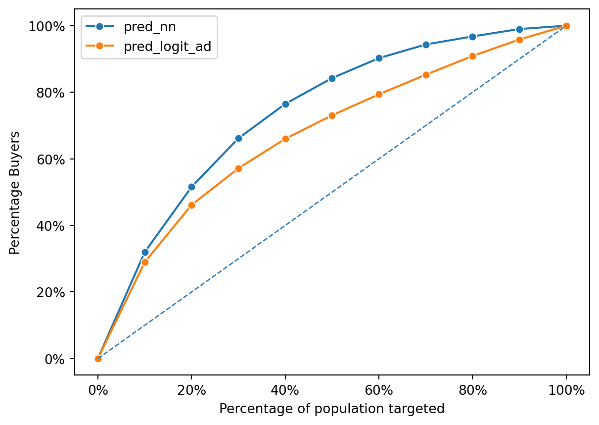
Based on the graph, the neural network is better because for any given percentage of customers, it captures a higher percentage of the total response compared to the logistic regression model.

In the neural network model, we use Grid Search to tune the hyperparameters, i.e. the hidden layer size and the learning rate. These two hyperparameters can influence the outcome:

• Hidden layer size: By finding the right balance through grid search, we can avoid overfitting or underfitting the model, leading to a model that generalizes well to new data.

• Learning rate: the learning rate controls how much the model’s weights are updated during training. Tuning the learning rate to a level that allows for efficient and effective learning is critical for good performance.

The combination of these two hyperparameters enables the neural network to capture the complexity of the data without overfitting, leading to better generalization and ultimately better performance on the gain chart.

# prediction on rnd_30k == 0 for neutral network "ad" model
pred = cg_ad_treatment[cg_ad_treatment['rnd_30k'] == 0]["pred_nn"]
actual = cg_ad_treatment[cg_ad_treatment['rnd_30k'] == 0]["converted_yes"]
fpr, tpr, thresholds = metrics.roc_curve(actual, pred)
metrics.auc(fpr, tpr).round(3)

0.782

# again, predict on rnd_30k == 0 for logistic regression "ad" model
pred = cg_ad_treatment[cg_ad_treatment['rnd_30k'] == 0]["pred_logit_ad"]
actual = cg_ad_treatment[cg_ad_treatment['rnd_30k'] == 0]["converted_yes"]
fpr, tpr, thresholds = metrics.roc_curve(actual, pred)
metrics.auc(fpr, tpr).round(3)

0.703

The AUC of the neural network model is 0.782 while the AUC of the logistic regression model is 0.703. Both models have good performance, but the difference in AUC shows that the neural netwrork model has a significant better performance in term of overall measure of accuracy across all thresholds. This confirms the visual interpretation from the gain chart, where the neural network model outperforms the logistic regression model.

Calculate the profit improvement of the neutral network ad

nn_group3 = cg_ad_treatment[cg_ad_treatment['rnd_30k'] == 0].nlargest(30000, 'pred_nn')
nn_response_rate, nn_profit = profit_calc(nn_group3)

/var/folders/28/cfl1_cfs3bb536qkz8wkys_w0000gn/T/ipykernel_5776/2151466375.py:2: FutureWarning:

Series.__getitem__ treating keys as positions is deprecated. In a future version, integer keys will always be treated as labels (consistent with DataFrame behavior). To access a value by position, use `ser.iloc[pos]`

mod_pef = pd.DataFrame({
    "model": ["Neural Network", "Ads"],
    "Response Rate": [nn_response_rate, ads_response_rate],
    "Profit": [nn_profit, ads_profit]
})
mod_pef

	model	Response Rate	Profit
0	Neural Network	0.311933	95276.42
1	Ads	0.273900	78172.83

profit_improvement = nn_profit - ads_profit
profit_improvement

17103.59000000004

That said, with the better performance of the neural network model, we can expect a better profit improvement compared to the logistic regression model. The profit improvement from using Neural Network model over the logistic regression model ad is $68,954, this represents a 22.05% improvement in profit when using Neural Network model over the logistic regression model ad.

Train and tune random forest model

rf = rsm.model.rforest(
    data = {'cg_ad_campaign': cg_ad_treatment[cg_ad_treatment['rnd_30k'] == 1]},
    rvar = 'converted_yes',
    evar = [
        "GameLevel",
        "NumGameDays",
        "NumGameDays4Plus",
        "NumInGameMessagesSent",
        "NumFriends",
        "NumFriendRequestIgnored",
        "NumSpaceHeroBadges",
        "AcquiredSpaceship",
        "AcquiredIonWeapon",
        "TimesLostSpaceship",
        "TimesKilled",
        "TimesCaptain",
        "TimesNavigator",
        "PurchasedCoinPackSmall",
        "PurchasedCoinPackLarge",
        "NumAdsClicked",
        "DaysUser",
        "UserConsole",
        "UserHasOldOS"
    ]
)
rf.summary()

Random Forest
Data                 : cg_ad_campaign
Response variable    : converted_yes
Level                : None
Explanatory variables: GameLevel, NumGameDays, NumGameDays4Plus, NumInGameMessagesSent, NumFriends, NumFriendRequestIgnored, NumSpaceHeroBadges, AcquiredSpaceship, AcquiredIonWeapon, TimesLostSpaceship, TimesKilled, TimesCaptain, TimesNavigator, PurchasedCoinPackSmall, PurchasedCoinPackLarge, NumAdsClicked, DaysUser, UserConsole, UserHasOldOS
OOB                  : True
Model type           : classification
Nr. of features      : (19, 19)
Nr. of observations  : 30,000
max_features         : sqrt (4)
n_estimators         : 100
min_samples_leaf     : 1
random_state         : 1234
AUC                  : 0.759

Estimation data      :
 GameLevel  NumGameDays  NumGameDays4Plus  NumInGameMessagesSent  NumFriends  NumFriendRequestIgnored  NumSpaceHeroBadges  TimesLostSpaceship  TimesKilled  TimesCaptain  TimesNavigator  NumAdsClicked  DaysUser  AcquiredSpaceship_yes  AcquiredIonWeapon_yes  PurchasedCoinPackSmall_yes  PurchasedCoinPackLarge_yes  UserConsole_yes  UserHasOldOS_yes
         2            8                 0                      0           4                        5                   0                   0            0             8               0              3      1889                  False                  False                        True                       False            False              True
         5           15                 0                    179         362                       50                   0                  22            0             4               4              2      1308                   True                  False                       False                       False             True             False
         7            7                 0                    267           0                       64                   0                   5            0             0               0              1      3562                  False                  False                       False                        True             True             False
         4            4                 0                     36           0                        0                   0                   0            0             0               0              2      2922                  False                  False                       False                       False             True             False
         8           17                 0                    222          20                       63                  10                  10            0             9               6              4      2192                   True                  False                        True                       False             True             False

Model Tuning

max_features = [None, 'auto', 'sqrt', 'log2', 0.25, 0.5, 0.75, 1.0, 2.0, 3.0, 4.0]
n_estimators = [10, 50, 100, 200, 500, 1000]

param_grid = {"max_features": max_features, "n_estimators": n_estimators}
scoring = {"AUC": "roc_auc"}

rf_cv = GridSearchCV(rf.fitted, param_grid, scoring=scoring, cv=5, n_jobs=4, refit="AUC", verbose=5)

rf.data_onehot.mean().round(3)
rf.data.converted_yes.mean()

0.13043333333333335

rf_cv.fit(rf.data_onehot, rf.data.converted_yes)

Fitting 5 folds for each of 66 candidates, totalling 330 fits
[CV 3/5] END hidden_layer_sizes=(1,), learning_rate_init=0.1; AUC: (test=0.714) total time=   0.1s
[CV 1/5] END hidden_layer_sizes=(1,), learning_rate_init=0.01; AUC: (test=0.696) total time=   0.2s
[CV 1/5] END hidden_layer_sizes=(1,), learning_rate_init=0.001; AUC: (test=0.696) total time=   0.2s
[CV 1/5] END hidden_layer_sizes=(1,), learning_rate_init=0.0001; AUC: (test=0.696) total time=   0.2s
[CV 5/5] END hidden_layer_sizes=(1,), learning_rate_init=0.0001; AUC: (test=0.702) total time=   0.2s
[CV 4/5] END hidden_layer_sizes=(2,), learning_rate_init=0.1; AUC: (test=0.752) total time=   0.8s
[CV 5/5] END hidden_layer_sizes=(2,), learning_rate_init=0.1; AUC: (test=0.759) total time=   1.6s
[CV 2/5] END hidden_layer_sizes=(2,), learning_rate_init=0.01; AUC: (test=0.745) total time=   3.4s
[CV 1/5] END hidden_layer_sizes=(2,), learning_rate_init=0.001; AUC: (test=0.747) total time=   6.2s
[CV 4/5] END hidden_layer_sizes=(2,), learning_rate_init=0.0001; AUC: (test=0.752) total time=   0.9s
[CV 5/5] END hidden_layer_sizes=(2,), learning_rate_init=0.0001; AUC: (test=0.759) total time=   2.1s
[CV 3/5] END hidden_layer_sizes=(3,), learning_rate_init=0.1; AUC: (test=0.767) total time=   6.5s
[CV 1/5] END hidden_layer_sizes=(3,), learning_rate_init=0.01; AUC: (test=0.750) total time=   9.5s
[CV 4/5] END hidden_layer_sizes=(3,), learning_rate_init=0.01; AUC: (test=0.726) total time=   0.9s
[CV 1/5] END hidden_layer_sizes=(3,), learning_rate_init=0.001; AUC: (test=0.750) total time=   9.0s
[CV 4/5] END hidden_layer_sizes=(3,), learning_rate_init=0.001; AUC: (test=0.726) total time=   0.7s
[CV 5/5] END hidden_layer_sizes=(3,), learning_rate_init=0.001; AUC: (test=0.758) total time=   7.4s
[CV 3/5] END hidden_layer_sizes=(3,), learning_rate_init=0.0001; AUC: (test=0.767) total time=   6.1s
[CV 1/5] END hidden_layer_sizes=(3, 3), learning_rate_init=0.1; AUC: (test=0.770) total time=  12.5s
[CV 5/5] END hidden_layer_sizes=(3, 3), learning_rate_init=0.1; AUC: (test=0.764) total time=  19.7s
[CV 5/5] END hidden_layer_sizes=(3, 3), learning_rate_init=0.01; AUC: (test=0.764) total time=  18.4s
[CV 5/5] END hidden_layer_sizes=(3, 3), learning_rate_init=0.001; AUC: (test=0.764) total time=  18.9s
[CV 5/5] END hidden_layer_sizes=(3, 3), learning_rate_init=0.0001; AUC: (test=0.764) total time=  19.5s
[CV 5/5] END hidden_layer_sizes=(4, 2), learning_rate_init=0.1; AUC: (test=0.779) total time=  12.3s
[CV 3/5] END hidden_layer_sizes=(4, 2), learning_rate_init=0.01; AUC: (test=0.788) total time=  21.0s
[CV 5/5] END hidden_layer_sizes=(4, 2), learning_rate_init=0.001; AUC: (test=0.779) total time=  11.5s
[CV 3/5] END hidden_layer_sizes=(4, 2), learning_rate_init=0.0001; AUC: (test=0.788) total time=  23.1s
[CV 4/5] END hidden_layer_sizes=(5, 5), learning_rate_init=0.1; AUC: (test=0.785) total time=  19.8s
[CV 1/5] END hidden_layer_sizes=(5, 5), learning_rate_init=0.01; AUC: (test=0.760) total time=  31.5s
[CV 5/5] END hidden_layer_sizes=(5, 5), learning_rate_init=0.01; AUC: (test=0.762) total time=  14.1s
[CV 1/5] END hidden_layer_sizes=(5, 5), learning_rate_init=0.001; AUC: (test=0.760) total time=  36.7s
[CV 5/5] END hidden_layer_sizes=(5, 5), learning_rate_init=0.001; AUC: (test=0.762) total time=  13.6s
[CV 2/5] END hidden_layer_sizes=(5, 5), learning_rate_init=0.0001; AUC: (test=0.778) total time=  49.5s
[CV 2/5] END max_features=None, n_estimators=10; AUC: (test=0.720) total time=   0.8s
[CV 5/5] END max_features=None, n_estimators=10; AUC: (test=0.720) total time=   0.8s
[CV 4/5] END max_features=None, n_estimators=50; AUC: (test=0.753) total time=   3.9s
[CV 3/5] END max_features=None, n_estimators=100; AUC: (test=0.767) total time=   7.6s
[CV 2/5] END max_features=None, n_estimators=200; AUC: (test=0.766) total time=  16.4s
[CV 1/5] END max_features=None, n_estimators=500; AUC: (test=0.761) total time=  38.6s
[CV 4/5] END hidden_layer_sizes=(1,), learning_rate_init=0.1; AUC: (test=0.698) total time=   0.2s
[CV 2/5] END hidden_layer_sizes=(1,), learning_rate_init=0.01; AUC: (test=0.712) total time=   0.1s
[CV 4/5] END hidden_layer_sizes=(1,), learning_rate_init=0.01; AUC: (test=0.698) total time=   0.2s
[CV 3/5] END hidden_layer_sizes=(1,), learning_rate_init=0.001; AUC: (test=0.714) total time=   0.1s
[CV 2/5] END hidden_layer_sizes=(1,), learning_rate_init=0.0001; AUC: (test=0.712) total time=   0.1s
[CV 1/5] END hidden_layer_sizes=(2,), learning_rate_init=0.1; AUC: (test=0.747) total time=   6.0s
[CV 5/5] END hidden_layer_sizes=(2,), learning_rate_init=0.01; AUC: (test=0.759) total time=   1.8s
[CV 3/5] END hidden_layer_sizes=(2,), learning_rate_init=0.001; AUC: (test=0.768) total time=   2.0s
[CV 1/5] END hidden_layer_sizes=(2,), learning_rate_init=0.0001; AUC: (test=0.747) total time=   6.5s
[CV 4/5] END hidden_layer_sizes=(3,), learning_rate_init=0.1; AUC: (test=0.726) total time=   0.8s
[CV 5/5] END hidden_layer_sizes=(3,), learning_rate_init=0.1; AUC: (test=0.758) total time=   7.3s
[CV 3/5] END hidden_layer_sizes=(3,), learning_rate_init=0.01; AUC: (test=0.767) total time=   7.0s
[CV 5/5] END hidden_layer_sizes=(3,), learning_rate_init=0.01; AUC: (test=0.758) total time=   7.7s
[CV 3/5] END hidden_layer_sizes=(3,), learning_rate_init=0.001; AUC: (test=0.767) total time=   6.7s
[CV 2/5] END hidden_layer_sizes=(3,), learning_rate_init=0.0001; AUC: (test=0.768) total time=  21.8s
[CV 4/5] END hidden_layer_sizes=(3, 3), learning_rate_init=0.1; AUC: (test=0.794) total time=  13.6s
[CV 2/5] END hidden_layer_sizes=(3, 3), learning_rate_init=0.01; AUC: (test=0.780) total time=  23.9s
[CV 4/5] END hidden_layer_sizes=(3, 3), learning_rate_init=0.001; AUC: (test=0.794) total time=  12.6s
[CV 2/5] END hidden_layer_sizes=(3, 3), learning_rate_init=0.0001; AUC: (test=0.780) total time=  23.9s
[CV 4/5] END hidden_layer_sizes=(4, 2), learning_rate_init=0.1; AUC: (test=0.792) total time=  11.2s
[CV 2/5] END hidden_layer_sizes=(4, 2), learning_rate_init=0.01; AUC: (test=0.780) total time=   5.3s
[CV 4/5] END hidden_layer_sizes=(4, 2), learning_rate_init=0.01; AUC: (test=0.792) total time=  10.7s
[CV 2/5] END hidden_layer_sizes=(4, 2), learning_rate_init=0.001; AUC: (test=0.780) total time=   5.2s
[CV 3/5] END hidden_layer_sizes=(4, 2), learning_rate_init=0.001; AUC: (test=0.788) total time=  21.8s
[CV 5/5] END hidden_layer_sizes=(4, 2), learning_rate_init=0.0001; AUC: (test=0.779) total time=  12.0s
[CV 3/5] END hidden_layer_sizes=(5, 5), learning_rate_init=0.1; AUC: (test=0.780) total time=  45.9s
[CV 3/5] END hidden_layer_sizes=(5, 5), learning_rate_init=0.01; AUC: (test=0.780) total time=  45.9s
[CV 3/5] END hidden_layer_sizes=(5, 5), learning_rate_init=0.001; AUC: (test=0.780) total time=  45.6s
[CV 4/5] END hidden_layer_sizes=(5, 5), learning_rate_init=0.0001; AUC: (test=0.785) total time=  20.6s
[CV 1/5] END max_features=None, n_estimators=10; AUC: (test=0.709) total time=   0.8s
[CV 2/5] END max_features=None, n_estimators=50; AUC: (test=0.757) total time=   3.8s
[CV 5/5] END max_features=None, n_estimators=50; AUC: (test=0.752) total time=   3.8s
[CV 4/5] END max_features=None, n_estimators=100; AUC: (test=0.758) total time=   7.6s
[CV 3/5] END max_features=None, n_estimators=200; AUC: (test=0.769) total time=  16.5s
[CV 2/5] END max_features=None, n_estimators=500; AUC: (test=0.768) total time=  38.4s
[CV 2/5] END hidden_layer_sizes=(1,), learning_rate_init=0.1; AUC: (test=0.712) total time=   0.1s
[CV 5/5] END hidden_layer_sizes=(1,), learning_rate_init=0.1; AUC: (test=0.702) total time=   0.2s
[CV 5/5] END hidden_layer_sizes=(1,), learning_rate_init=0.01; AUC: (test=0.702) total time=   0.2s
[CV 5/5] END hidden_layer_sizes=(1,), learning_rate_init=0.001; AUC: (test=0.702) total time=   0.2s
[CV 4/5] END hidden_layer_sizes=(1,), learning_rate_init=0.0001; AUC: (test=0.698) total time=   0.1s
[CV 3/5] END hidden_layer_sizes=(2,), learning_rate_init=0.1; AUC: (test=0.768) total time=   2.1s
[CV 1/5] END hidden_layer_sizes=(2,), learning_rate_init=0.01; AUC: (test=0.747) total time=   6.4s
[CV 4/5] END hidden_layer_sizes=(2,), learning_rate_init=0.001; AUC: (test=0.752) total time=   0.8s
[CV 5/5] END hidden_layer_sizes=(2,), learning_rate_init=0.001; AUC: (test=0.759) total time=   1.7s
[CV 3/5] END hidden_layer_sizes=(2,), learning_rate_init=0.0001; AUC: (test=0.768) total time=   2.3s
[CV 1/5] END hidden_layer_sizes=(3,), learning_rate_init=0.1; AUC: (test=0.750) total time=   8.8s
[CV 2/5] END hidden_layer_sizes=(3,), learning_rate_init=0.01; AUC: (test=0.768) total time=  23.3s
[CV 1/5] END hidden_layer_sizes=(3,), learning_rate_init=0.0001; AUC: (test=0.750) total time=   8.3s
[CV 4/5] END hidden_layer_sizes=(3,), learning_rate_init=0.0001; AUC: (test=0.726) total time=   0.8s
[CV 5/5] END hidden_layer_sizes=(3,), learning_rate_init=0.0001; AUC: (test=0.758) total time=   7.2s
[CV 3/5] END hidden_layer_sizes=(3, 3), learning_rate_init=0.1; AUC: (test=0.764) total time=   6.9s
[CV 1/5] END hidden_layer_sizes=(3, 3), learning_rate_init=0.01; AUC: (test=0.770) total time=  12.9s
[CV 3/5] END hidden_layer_sizes=(3, 3), learning_rate_init=0.01; AUC: (test=0.764) total time=   6.9s
[CV 1/5] END hidden_layer_sizes=(3, 3), learning_rate_init=0.001; AUC: (test=0.770) total time=  13.0s
[CV 3/5] END hidden_layer_sizes=(3, 3), learning_rate_init=0.001; AUC: (test=0.764) total time=   6.6s
[CV 1/5] END hidden_layer_sizes=(3, 3), learning_rate_init=0.0001; AUC: (test=0.770) total time=  12.2s
[CV 3/5] END hidden_layer_sizes=(3, 3), learning_rate_init=0.0001; AUC: (test=0.764) total time=   7.1s
[CV 1/5] END hidden_layer_sizes=(4, 2), learning_rate_init=0.1; AUC: (test=0.771) total time=  18.7s
[CV 1/5] END hidden_layer_sizes=(4, 2), learning_rate_init=0.01; AUC: (test=0.771) total time=  18.0s
[CV 1/5] END hidden_layer_sizes=(4, 2), learning_rate_init=0.001; AUC: (test=0.771) total time=  17.3s
[CV 1/5] END hidden_layer_sizes=(4, 2), learning_rate_init=0.0001; AUC: (test=0.771) total time=  17.0s
[CV 1/5] END hidden_layer_sizes=(5, 5), learning_rate_init=0.1; AUC: (test=0.760) total time=  31.9s
[CV 5/5] END hidden_layer_sizes=(5, 5), learning_rate_init=0.1; AUC: (test=0.762) total time=  13.8s
[CV 2/5] END hidden_layer_sizes=(5, 5), learning_rate_init=0.01; AUC: (test=0.778) total time=  58.0s
[CV 4/5] END hidden_layer_sizes=(5, 5), learning_rate_init=0.001; AUC: (test=0.785) total time=  23.5s
[CV 1/5] END hidden_layer_sizes=(5, 5), learning_rate_init=0.0001; AUC: (test=0.760) total time=  32.5s
[CV 5/5] END hidden_layer_sizes=(5, 5), learning_rate_init=0.0001; AUC: (test=0.762) total time=  12.7s
[CV 4/5] END max_features=None, n_estimators=10; AUC: (test=0.711) total time=   0.8s
[CV 3/5] END max_features=None, n_estimators=50; AUC: (test=0.764) total time=   3.8s
[CV 2/5] END max_features=None, n_estimators=100; AUC: (test=0.764) total time=   7.5s
[CV 5/5] END max_features=None, n_estimators=100; AUC: (test=0.758) total time=   7.5s
[CV 4/5] END max_features=None, n_estimators=200; AUC: (test=0.762) total time=  16.8s
[CV 3/5] END max_features=None, n_estimators=500; AUC: (test=0.772) total time=  38.5s
[CV 1/5] END hidden_layer_sizes=(1,), learning_rate_init=0.1; AUC: (test=0.696) total time=   0.2s
[CV 3/5] END hidden_layer_sizes=(1,), learning_rate_init=0.01; AUC: (test=0.714) total time=   0.1s
[CV 2/5] END hidden_layer_sizes=(1,), learning_rate_init=0.001; AUC: (test=0.712) total time=   0.2s
[CV 4/5] END hidden_layer_sizes=(1,), learning_rate_init=0.001; AUC: (test=0.698) total time=   0.2s
[CV 3/5] END hidden_layer_sizes=(1,), learning_rate_init=0.0001; AUC: (test=0.714) total time=   0.1s
[CV 2/5] END hidden_layer_sizes=(2,), learning_rate_init=0.1; AUC: (test=0.745) total time=   3.5s
[CV 3/5] END hidden_layer_sizes=(2,), learning_rate_init=0.01; AUC: (test=0.768) total time=   2.3s
[CV 4/5] END hidden_layer_sizes=(2,), learning_rate_init=0.01; AUC: (test=0.752) total time=   0.7s
[CV 2/5] END hidden_layer_sizes=(2,), learning_rate_init=0.001; AUC: (test=0.745) total time=   3.7s
[CV 2/5] END hidden_layer_sizes=(2,), learning_rate_init=0.0001; AUC: (test=0.745) total time=   3.8s
[CV 2/5] END hidden_layer_sizes=(3,), learning_rate_init=0.1; AUC: (test=0.768) total time=  23.3s
[CV 2/5] END hidden_layer_sizes=(3,), learning_rate_init=0.001; AUC: (test=0.768) total time=  21.9s
[CV 2/5] END hidden_layer_sizes=(3, 3), learning_rate_init=0.1; AUC: (test=0.780) total time=  23.5s
[CV 4/5] END hidden_layer_sizes=(3, 3), learning_rate_init=0.01; AUC: (test=0.794) total time=  14.5s
[CV 2/5] END hidden_layer_sizes=(3, 3), learning_rate_init=0.001; AUC: (test=0.780) total time=  23.5s
[CV 4/5] END hidden_layer_sizes=(3, 3), learning_rate_init=0.0001; AUC: (test=0.794) total time=  14.2s
[CV 2/5] END hidden_layer_sizes=(4, 2), learning_rate_init=0.1; AUC: (test=0.780) total time=   5.2s
[CV 3/5] END hidden_layer_sizes=(4, 2), learning_rate_init=0.1; AUC: (test=0.788) total time=  22.6s
[CV 5/5] END hidden_layer_sizes=(4, 2), learning_rate_init=0.01; AUC: (test=0.779) total time=  11.5s
[CV 4/5] END hidden_layer_sizes=(4, 2), learning_rate_init=0.001; AUC: (test=0.792) total time=  10.7s
[CV 2/5] END hidden_layer_sizes=(4, 2), learning_rate_init=0.0001; AUC: (test=0.780) total time=   5.2s
[CV 4/5] END hidden_layer_sizes=(4, 2), learning_rate_init=0.0001; AUC: (test=0.792) total time=  11.0s
[CV 2/5] END hidden_layer_sizes=(5, 5), learning_rate_init=0.1; AUC: (test=0.778) total time=  59.3s
[CV 4/5] END hidden_layer_sizes=(5, 5), learning_rate_init=0.01; AUC: (test=0.785) total time=  21.2s
[CV 2/5] END hidden_layer_sizes=(5, 5), learning_rate_init=0.001; AUC: (test=0.778) total time= 1.0min
[CV 3/5] END hidden_layer_sizes=(5, 5), learning_rate_init=0.0001; AUC: (test=0.780) total time=  36.1s
[CV 3/5] END max_features=None, n_estimators=10; AUC: (test=0.727) total time=   0.8s
[CV 1/5] END max_features=None, n_estimators=50; AUC: (test=0.752) total time=   3.9s
[CV 1/5] END max_features=None, n_estimators=100; AUC: (test=0.757) total time=   7.6s
[CV 1/5] END max_features=None, n_estimators=200; AUC: (test=0.759) total time=  16.6s
[CV 5/5] END max_features=None, n_estimators=200; AUC: (test=0.761) total time=  15.4s
[CV 4/5] END max_features=None, n_estimators=500; AUC: (test=0.765) total time=  38.6s
[CV 5/5] END max_features=None, n_estimators=500; AUC: (test=0.764) total time=  39.1s
[CV 4/5] END max_features=None, n_estimators=1000; AUC: (test=0.765) total time= 1.4min
[CV 3/5] END max_features=sqrt, n_estimators=500; AUC: (test=0.787) total time=  11.4s
[CV 1/5] END max_features=sqrt, n_estimators=1000; AUC: (test=0.772) total time=  23.0s
[CV 3/5] END max_features=None, n_estimators=1000; AUC: (test=0.772) total time= 1.4min
[CV 2/5] END max_features=sqrt, n_estimators=100; AUC: (test=0.776) total time=   2.2s
[CV 4/5] END max_features=sqrt, n_estimators=100; AUC: (test=0.766) total time=   2.2s
[CV 5/5] END max_features=sqrt, n_estimators=100; AUC: (test=0.770) total time=   2.3s
[CV 2/5] END max_features=sqrt, n_estimators=200; AUC: (test=0.781) total time=   4.8s
[CV 4/5] END max_features=sqrt, n_estimators=200; AUC: (test=0.774) total time=   4.6s
[CV 1/5] END max_features=sqrt, n_estimators=500; AUC: (test=0.771) total time=  11.0s
[CV 4/5] END max_features=sqrt, n_estimators=500; AUC: (test=0.779) total time=  11.6s
[CV 2/5] END max_features=sqrt, n_estimators=1000; AUC: (test=0.782) total time=  23.1s
[CV 2/5] END max_features=None, n_estimators=1000; AUC: (test=0.768) total time= 1.3min
[CV 1/5] END max_features=auto, n_estimators=10; AUC: (test=nan) total time=   0.0s
[CV 2/5] END max_features=auto, n_estimators=10; AUC: (test=nan) total time=   0.0s
[CV 3/5] END max_features=auto, n_estimators=10; AUC: (test=nan) total time=   0.0s
[CV 4/5] END max_features=auto, n_estimators=10; AUC: (test=nan) total time=   0.0s
[CV 5/5] END max_features=auto, n_estimators=10; AUC: (test=nan) total time=   0.0s
[CV 1/5] END max_features=auto, n_estimators=50; AUC: (test=nan) total time=   0.0s
[CV 2/5] END max_features=auto, n_estimators=50; AUC: (test=nan) total time=   0.0s
[CV 3/5] END max_features=auto, n_estimators=50; AUC: (test=nan) total time=   0.0s
[CV 4/5] END max_features=auto, n_estimators=50; AUC: (test=nan) total time=   0.0s
[CV 5/5] END max_features=auto, n_estimators=50; AUC: (test=nan) total time=   0.0s
[CV 1/5] END max_features=auto, n_estimators=100; AUC: (test=nan) total time=   0.0s
[CV 2/5] END max_features=auto, n_estimators=100; AUC: (test=nan) total time=   0.0s
[CV 3/5] END max_features=auto, n_estimators=100; AUC: (test=nan) total time=   0.0s
[CV 4/5] END max_features=auto, n_estimators=100; AUC: (test=nan) total time=   0.0s
[CV 5/5] END max_features=auto, n_estimators=100; AUC: (test=nan) total time=   0.0s
[CV 1/5] END max_features=auto, n_estimators=200; AUC: (test=nan) total time=   0.0s
[CV 2/5] END max_features=auto, n_estimators=200; AUC: (test=nan) total time=   0.0s
[CV 3/5] END max_features=auto, n_estimators=200; AUC: (test=nan) total time=   0.0s
[CV 4/5] END max_features=auto, n_estimators=200; AUC: (test=nan) total time=   0.0s
[CV 5/5] END max_features=auto, n_estimators=200; AUC: (test=nan) total time=   0.0s
[CV 1/5] END max_features=auto, n_estimators=500; AUC: (test=nan) total time=   0.0s
[CV 2/5] END max_features=auto, n_estimators=500; AUC: (test=nan) total time=   0.0s
[CV 3/5] END max_features=auto, n_estimators=500; AUC: (test=nan) total time=   0.0s
[CV 4/5] END max_features=auto, n_estimators=500; AUC: (test=nan) total time=   0.0s
[CV 5/5] END max_features=auto, n_estimators=500; AUC: (test=nan) total time=   0.0s
[CV 1/5] END max_features=auto, n_estimators=1000; AUC: (test=nan) total time=   0.0s
[CV 2/5] END max_features=auto, n_estimators=1000; AUC: (test=nan) total time=   0.0s
[CV 3/5] END max_features=auto, n_estimators=1000; AUC: (test=nan) total time=   0.0s
[CV 4/5] END max_features=auto, n_estimators=1000; AUC: (test=nan) total time=   0.0s
[CV 5/5] END max_features=auto, n_estimators=1000; AUC: (test=nan) total time=   0.0s
[CV 1/5] END max_features=sqrt, n_estimators=10; AUC: (test=0.717) total time=   0.3s
[CV 2/5] END max_features=sqrt, n_estimators=10; AUC: (test=0.720) total time=   0.2s
[CV 3/5] END max_features=sqrt, n_estimators=10; AUC: (test=0.725) total time=   0.2s
[CV 4/5] END max_features=sqrt, n_estimators=10; AUC: (test=0.708) total time=   0.4s
[CV 5/5] END max_features=sqrt, n_estimators=10; AUC: (test=0.713) total time=   0.2s
[CV 1/5] END max_features=sqrt, n_estimators=50; AUC: (test=0.760) total time=   1.2s
[CV 2/5] END max_features=sqrt, n_estimators=50; AUC: (test=0.764) total time=   1.4s
[CV 3/5] END max_features=sqrt, n_estimators=50; AUC: (test=0.775) total time=   1.2s
[CV 4/5] END max_features=sqrt, n_estimators=50; AUC: (test=0.757) total time=   1.2s
[CV 5/5] END max_features=sqrt, n_estimators=50; AUC: (test=0.766) total time=   1.2s
[CV 1/5] END max_features=sqrt, n_estimators=100; AUC: (test=0.767) total time=   2.3s
[CV 3/5] END max_features=sqrt, n_estimators=100; AUC: (test=0.781) total time=   2.3s
[CV 1/5] END max_features=sqrt, n_estimators=200; AUC: (test=0.771) total time=   4.9s
[CV 3/5] END max_features=sqrt, n_estimators=200; AUC: (test=0.784) total time=   4.7s
[CV 5/5] END max_features=sqrt, n_estimators=200; AUC: (test=0.776) total time=   4.6s
[CV 2/5] END max_features=sqrt, n_estimators=500; AUC: (test=0.781) total time=  11.6s
[CV 5/5] END max_features=sqrt, n_estimators=500; AUC: (test=0.777) total time=  11.4s
[CV 3/5] END max_features=sqrt, n_estimators=1000; AUC: (test=0.789) total time=  23.2s
[CV 1/5] END max_features=log2, n_estimators=10; AUC: (test=0.717) total time=   0.2s
[CV 3/5] END max_features=log2, n_estimators=10; AUC: (test=0.725) total time=   0.2s
[CV 5/5] END max_features=log2, n_estimators=10; AUC: (test=0.713) total time=   0.2s
[CV 2/5] END max_features=log2, n_estimators=50; AUC: (test=0.764) total time=   1.1s
[CV 4/5] END max_features=log2, n_estimators=50; AUC: (test=0.757) total time=   1.1s
[CV 1/5] END max_features=log2, n_estimators=100; AUC: (test=0.767) total time=   2.3s
[CV 3/5] END max_features=log2, n_estimators=100; AUC: (test=0.781) total time=   2.3s
[CV 5/5] END max_features=log2, n_estimators=100; AUC: (test=0.770) total time=   2.5s
[CV 2/5] END max_features=log2, n_estimators=200; AUC: (test=0.781) total time=   4.5s
[CV 4/5] END max_features=log2, n_estimators=200; AUC: (test=0.774) total time=   4.5s
[CV 2/5] END max_features=log2, n_estimators=500; AUC: (test=0.781) total time=  11.0s

/Users/duyentran/Library/Python/3.11/lib/python/site-packages/sklearn/ensemble/_forest.py:615: UserWarning: Some inputs do not have OOB scores. This probably means too few trees were used to compute any reliable OOB estimates.
  warn(
/Users/duyentran/Library/Python/3.11/lib/python/site-packages/sklearn/ensemble/_forest.py:615: UserWarning: Some inputs do not have OOB scores. This probably means too few trees were used to compute any reliable OOB estimates.
  warn(
/Users/duyentran/Library/Python/3.11/lib/python/site-packages/sklearn/ensemble/_forest.py:615: UserWarning: Some inputs do not have OOB scores. This probably means too few trees were used to compute any reliable OOB estimates.
  warn(
/Users/duyentran/Library/Python/3.11/lib/python/site-packages/sklearn/ensemble/_forest.py:615: UserWarning: Some inputs do not have OOB scores. This probably means too few trees were used to compute any reliable OOB estimates.
  warn(
/Users/duyentran/Library/Python/3.11/lib/python/site-packages/sklearn/ensemble/_forest.py:615: UserWarning: Some inputs do not have OOB scores. This probably means too few trees were used to compute any reliable OOB estimates.
  warn(
/Users/duyentran/Library/Python/3.11/lib/python/site-packages/joblib/externals/loky/process_executor.py:752: UserWarning:

A worker stopped while some jobs were given to the executor. This can be caused by a too short worker timeout or by a memory leak.

/Users/duyentran/Library/Python/3.11/lib/python/site-packages/sklearn/ensemble/_forest.py:615: UserWarning: Some inputs do not have OOB scores. This probably means too few trees were used to compute any reliable OOB estimates.
  warn(
/Users/duyentran/Library/Python/3.11/lib/python/site-packages/sklearn/ensemble/_forest.py:615: UserWarning: Some inputs do not have OOB scores. This probably means too few trees were used to compute any reliable OOB estimates.
  warn(
/Users/duyentran/Library/Python/3.11/lib/python/site-packages/sklearn/ensemble/_forest.py:615: UserWarning: Some inputs do not have OOB scores. This probably means too few trees were used to compute any reliable OOB estimates.
  warn(
/Users/duyentran/Library/Python/3.11/lib/python/site-packages/sklearn/ensemble/_forest.py:615: UserWarning: Some inputs do not have OOB scores. This probably means too few trees were used to compute any reliable OOB estimates.
  warn(
/Users/duyentran/Library/Python/3.11/lib/python/site-packages/sklearn/ensemble/_forest.py:615: UserWarning: Some inputs do not have OOB scores. This probably means too few trees were used to compute any reliable OOB estimates.
  warn(
/Users/duyentran/Library/Python/3.11/lib/python/site-packages/sklearn/ensemble/_forest.py:615: UserWarning: Some inputs do not have OOB scores. This probably means too few trees were used to compute any reliable OOB estimates.
  warn(
/Users/duyentran/Library/Python/3.11/lib/python/site-packages/sklearn/ensemble/_forest.py:615: UserWarning: Some inputs do not have OOB scores. This probably means too few trees were used to compute any reliable OOB estimates.
  warn(
/Users/duyentran/Library/Python/3.11/lib/python/site-packages/sklearn/ensemble/_forest.py:615: UserWarning: Some inputs do not have OOB scores. This probably means too few trees were used to compute any reliable OOB estimates.
  warn(
/Users/duyentran/Library/Python/3.11/lib/python/site-packages/sklearn/ensemble/_forest.py:615: UserWarning: Some inputs do not have OOB scores. This probably means too few trees were used to compute any reliable OOB estimates.
  warn(
/Users/duyentran/Library/Python/3.11/lib/python/site-packages/sklearn/ensemble/_forest.py:615: UserWarning: Some inputs do not have OOB scores. This probably means too few trees were used to compute any reliable OOB estimates.
  warn(
/Users/duyentran/Library/Python/3.11/lib/python/site-packages/sklearn/ensemble/_forest.py:615: UserWarning: Some inputs do not have OOB scores. This probably means too few trees were used to compute any reliable OOB estimates.
  warn(
/Users/duyentran/Library/Python/3.11/lib/python/site-packages/sklearn/ensemble/_forest.py:615: UserWarning: Some inputs do not have OOB scores. This probably means too few trees were used to compute any reliable OOB estimates.
  warn(
/Users/duyentran/Library/Python/3.11/lib/python/site-packages/sklearn/ensemble/_forest.py:615: UserWarning: Some inputs do not have OOB scores. This probably means too few trees were used to compute any reliable OOB estimates.
  warn(
/Users/duyentran/Library/Python/3.11/lib/python/site-packages/sklearn/ensemble/_forest.py:615: UserWarning: Some inputs do not have OOB scores. This probably means too few trees were used to compute any reliable OOB estimates.
  warn(
/Users/duyentran/Library/Python/3.11/lib/python/site-packages/sklearn/ensemble/_forest.py:615: UserWarning: Some inputs do not have OOB scores. This probably means too few trees were used to compute any reliable OOB estimates.
  warn(
/Users/duyentran/Library/Python/3.11/lib/python/site-packages/sklearn/ensemble/_forest.py:615: UserWarning: Some inputs do not have OOB scores. This probably means too few trees were used to compute any reliable OOB estimates.
  warn(
/Users/duyentran/Library/Python/3.11/lib/python/site-packages/sklearn/ensemble/_forest.py:615: UserWarning: Some inputs do not have OOB scores. This probably means too few trees were used to compute any reliable OOB estimates.
  warn(
/Users/duyentran/Library/Python/3.11/lib/python/site-packages/sklearn/ensemble/_forest.py:615: UserWarning: Some inputs do not have OOB scores. This probably means too few trees were used to compute any reliable OOB estimates.
  warn(
/Users/duyentran/Library/Python/3.11/lib/python/site-packages/sklearn/ensemble/_forest.py:615: UserWarning: Some inputs do not have OOB scores. This probably means too few trees were used to compute any reliable OOB estimates.
  warn(
/Users/duyentran/Library/Python/3.11/lib/python/site-packages/sklearn/ensemble/_forest.py:615: UserWarning: Some inputs do not have OOB scores. This probably means too few trees were used to compute any reliable OOB estimates.
  warn(
/Users/duyentran/Library/Python/3.11/lib/python/site-packages/sklearn/ensemble/_forest.py:615: UserWarning: Some inputs do not have OOB scores. This probably means too few trees were used to compute any reliable OOB estimates.
  warn(
/Users/duyentran/Library/Python/3.11/lib/python/site-packages/sklearn/ensemble/_forest.py:615: UserWarning: Some inputs do not have OOB scores. This probably means too few trees were used to compute any reliable OOB estimates.
  warn(
/Users/duyentran/Library/Python/3.11/lib/python/site-packages/sklearn/ensemble/_forest.py:615: UserWarning: Some inputs do not have OOB scores. This probably means too few trees were used to compute any reliable OOB estimates.
  warn(
/Users/duyentran/Library/Python/3.11/lib/python/site-packages/sklearn/ensemble/_forest.py:615: UserWarning: Some inputs do not have OOB scores. This probably means too few trees were used to compute any reliable OOB estimates.
  warn(
/Users/duyentran/Library/Python/3.11/lib/python/site-packages/sklearn/ensemble/_forest.py:615: UserWarning: Some inputs do not have OOB scores. This probably means too few trees were used to compute any reliable OOB estimates.
  warn(
/Users/duyentran/Library/Python/3.11/lib/python/site-packages/sklearn/ensemble/_forest.py:615: UserWarning: Some inputs do not have OOB scores. This probably means too few trees were used to compute any reliable OOB estimates.
  warn(
/Users/duyentran/Library/Python/3.11/lib/python/site-packages/sklearn/ensemble/_forest.py:615: UserWarning: Some inputs do not have OOB scores. This probably means too few trees were used to compute any reliable OOB estimates.
  warn(
/Users/duyentran/Library/Python/3.11/lib/python/site-packages/sklearn/ensemble/_forest.py:615: UserWarning: Some inputs do not have OOB scores. This probably means too few trees were used to compute any reliable OOB estimates.
  warn(
/Users/duyentran/Library/Python/3.11/lib/python/site-packages/sklearn/ensemble/_forest.py:615: UserWarning: Some inputs do not have OOB scores. This probably means too few trees were used to compute any reliable OOB estimates.
  warn(
/Users/duyentran/Library/Python/3.11/lib/python/site-packages/sklearn/ensemble/_forest.py:615: UserWarning: Some inputs do not have OOB scores. This probably means too few trees were used to compute any reliable OOB estimates.
  warn(
/Users/duyentran/Library/Python/3.11/lib/python/site-packages/sklearn/model_selection/_validation.py:547: FitFailedWarning:


120 fits failed out of a total of 330.
The score on these train-test partitions for these parameters will be set to nan.
If these failures are not expected, you can try to debug them by setting error_score='raise'.

Below are more details about the failures:
--------------------------------------------------------------------------------
30 fits failed with the following error:
Traceback (most recent call last):
  File "/Users/duyentran/Library/Python/3.11/lib/python/site-packages/sklearn/model_selection/_validation.py", line 895, in _fit_and_score
    estimator.fit(X_train, y_train, **fit_params)
  File "/Users/duyentran/Library/Python/3.11/lib/python/site-packages/sklearn/base.py", line 1467, in wrapper
    estimator._validate_params()
  File "/Users/duyentran/Library/Python/3.11/lib/python/site-packages/sklearn/base.py", line 666, in _validate_params
    validate_parameter_constraints(
  File "/Users/duyentran/Library/Python/3.11/lib/python/site-packages/sklearn/utils/_param_validation.py", line 95, in validate_parameter_constraints
    raise InvalidParameterError(
sklearn.utils._param_validation.InvalidParameterError: The 'max_features' parameter of RandomForestClassifier must be an int in the range [1, inf), a float in the range (0.0, 1.0], a str among {'log2', 'sqrt'} or None. Got 'auto' instead.

--------------------------------------------------------------------------------
30 fits failed with the following error:
Traceback (most recent call last):
  File "/Users/duyentran/Library/Python/3.11/lib/python/site-packages/sklearn/model_selection/_validation.py", line 895, in _fit_and_score
    estimator.fit(X_train, y_train, **fit_params)
  File "/Users/duyentran/Library/Python/3.11/lib/python/site-packages/sklearn/base.py", line 1467, in wrapper
    estimator._validate_params()
  File "/Users/duyentran/Library/Python/3.11/lib/python/site-packages/sklearn/base.py", line 666, in _validate_params
    validate_parameter_constraints(
  File "/Users/duyentran/Library/Python/3.11/lib/python/site-packages/sklearn/utils/_param_validation.py", line 95, in validate_parameter_constraints
    raise InvalidParameterError(
sklearn.utils._param_validation.InvalidParameterError: The 'max_features' parameter of RandomForestClassifier must be an int in the range [1, inf), a float in the range (0.0, 1.0], a str among {'log2', 'sqrt'} or None. Got 2.0 instead.

--------------------------------------------------------------------------------
30 fits failed with the following error:
Traceback (most recent call last):
  File "/Users/duyentran/Library/Python/3.11/lib/python/site-packages/sklearn/model_selection/_validation.py", line 895, in _fit_and_score
    estimator.fit(X_train, y_train, **fit_params)
  File "/Users/duyentran/Library/Python/3.11/lib/python/site-packages/sklearn/base.py", line 1467, in wrapper
    estimator._validate_params()
  File "/Users/duyentran/Library/Python/3.11/lib/python/site-packages/sklearn/base.py", line 666, in _validate_params
    validate_parameter_constraints(
  File "/Users/duyentran/Library/Python/3.11/lib/python/site-packages/sklearn/utils/_param_validation.py", line 95, in validate_parameter_constraints
    raise InvalidParameterError(
sklearn.utils._param_validation.InvalidParameterError: The 'max_features' parameter of RandomForestClassifier must be an int in the range [1, inf), a float in the range (0.0, 1.0], a str among {'log2', 'sqrt'} or None. Got 3.0 instead.

--------------------------------------------------------------------------------
30 fits failed with the following error:
Traceback (most recent call last):
  File "/Users/duyentran/Library/Python/3.11/lib/python/site-packages/sklearn/model_selection/_validation.py", line 895, in _fit_and_score
    estimator.fit(X_train, y_train, **fit_params)
  File "/Users/duyentran/Library/Python/3.11/lib/python/site-packages/sklearn/base.py", line 1467, in wrapper
    estimator._validate_params()
  File "/Users/duyentran/Library/Python/3.11/lib/python/site-packages/sklearn/base.py", line 666, in _validate_params
    validate_parameter_constraints(
  File "/Users/duyentran/Library/Python/3.11/lib/python/site-packages/sklearn/utils/_param_validation.py", line 95, in validate_parameter_constraints
    raise InvalidParameterError(
sklearn.utils._param_validation.InvalidParameterError: The 'max_features' parameter of RandomForestClassifier must be an int in the range [1, inf), a float in the range (0.0, 1.0], a str among {'log2', 'sqrt'} or None. Got 4.0 instead.


/Users/duyentran/Library/Python/3.11/lib/python/site-packages/sklearn/model_selection/_search.py:1051: UserWarning:

One or more of the test scores are non-finite: [0.71732593 0.75550047 0.76098577 0.76354732 0.76619619 0.7663353
        nan        nan        nan        nan        nan        nan
 0.71661193 0.76449763 0.7718989  0.77712755 0.77905288 0.78021496
 0.71661193 0.76449763 0.7718989  0.77712755 0.77905288 0.78021496
 0.71661193 0.76449763 0.7718989  0.77712755 0.77905288 0.78021496
 0.71795268 0.76238447 0.76870114 0.77133255 0.77269637 0.77393492
 0.71287995 0.75707753 0.76285869 0.76608659 0.76859789 0.76972414
 0.71732593 0.75550047 0.76098577 0.76354732 0.76619619 0.7663353
        nan        nan        nan        nan        nan        nan
        nan        nan        nan        nan        nan        nan
        nan        nan        nan        nan        nan        nan]

GridSearchCV(cv=5,
             estimator=RandomForestClassifier(oob_score=True,
                                              random_state=1234),
             n_jobs=4,
             param_grid={'max_features': [None, 'auto', 'sqrt', 'log2', 0.25,
                                          0.5, 0.75, 1.0, 2.0, 3.0, 4.0],
                         'n_estimators': [10, 50, 100, 200, 500, 1000]},
             refit='AUC', scoring={'AUC': 'roc_auc'}, verbose=5)

In a Jupyter environment, please rerun this cell to show the HTML representation or trust the notebook.
On GitHub, the HTML representation is unable to render, please try loading this page with nbviewer.org.

rf_cv.best_params_

{'max_features': 'sqrt', 'n_estimators': 1000}

Retrain the model with the best hyperparameters

rf = rsm.model.rforest(
    data = {'cg_ad_campaign': cg_ad_treatment[cg_ad_treatment['rnd_30k'] == 1]},
    rvar = 'converted_yes',
    evar = [
        "GameLevel",
        "NumGameDays",
        "NumGameDays4Plus",
        "NumInGameMessagesSent",
        "NumFriends",
        "NumFriendRequestIgnored",
        "NumSpaceHeroBadges",
        "AcquiredSpaceship",
        "AcquiredIonWeapon",
        "TimesLostSpaceship",
        "TimesKilled",
        "TimesCaptain",
        "TimesNavigator",
        "PurchasedCoinPackSmall",
        "PurchasedCoinPackLarge",
        "NumAdsClicked",
        "DaysUser",
        "UserConsole",
        "UserHasOldOS"
    ],
    n_estimators = 1000,
    max_features = 0.25,
)
rf.summary()

Random Forest
Data                 : cg_ad_campaign
Response variable    : converted_yes
Level                : None
Explanatory variables: GameLevel, NumGameDays, NumGameDays4Plus, NumInGameMessagesSent, NumFriends, NumFriendRequestIgnored, NumSpaceHeroBadges, AcquiredSpaceship, AcquiredIonWeapon, TimesLostSpaceship, TimesKilled, TimesCaptain, TimesNavigator, PurchasedCoinPackSmall, PurchasedCoinPackLarge, NumAdsClicked, DaysUser, UserConsole, UserHasOldOS
OOB                  : True
Model type           : classification
Nr. of features      : (19, 19)
Nr. of observations  : 30,000
max_features         : 0.25 (0)
n_estimators         : 1000
min_samples_leaf     : 1
random_state         : 1234
AUC                  : 0.78

Estimation data      :
 GameLevel  NumGameDays  NumGameDays4Plus  NumInGameMessagesSent  NumFriends  NumFriendRequestIgnored  NumSpaceHeroBadges  TimesLostSpaceship  TimesKilled  TimesCaptain  TimesNavigator  NumAdsClicked  DaysUser  AcquiredSpaceship_yes  AcquiredIonWeapon_yes  PurchasedCoinPackSmall_yes  PurchasedCoinPackLarge_yes  UserConsole_yes  UserHasOldOS_yes
         2            8                 0                      0           4                        5                   0                   0            0             8               0              3      1889                  False                  False                        True                       False            False              True
         5           15                 0                    179         362                       50                   0                  22            0             4               4              2      1308                   True                  False                       False                       False             True             False
         7            7                 0                    267           0                       64                   0                   5            0             0               0              1      3562                  False                  False                       False                        True             True             False
         4            4                 0                     36           0                        0                   0                   0            0             0               0              2      2922                  False                  False                       False                       False             True             False
         8           17                 0                    222          20                       63                  10                  10            0             9               6              4      2192                   True                  False                        True                       False             True             False

cg_ad_treatment['pred_rf'] = rf.predict(cg_ad_treatment)['prediction']

fig = rsm.gains_plot(
    cg_ad_treatment[cg_ad_treatment['rnd_30k'] == 0],
    "converted", "yes",
    ["pred_logit_ad", "pred_rf"]
)

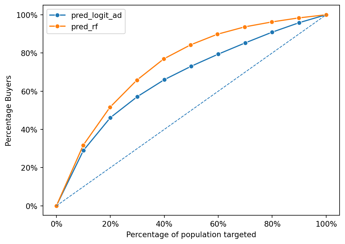
At the initial stages (when a small percentage of the population is targeted), the random forest model captures a higher percentage of the total response compared to the logistic regression model. This suggest that the random forest model is better at capturing the response in the early stages of targeting.

As more the population is targeted, both models’ curves flatten out, which is expected as the company each out to less likely buyers, the gain from each additional percentage of the population targeted decreases. However, the random forest model, which has been fine-tuned using grid search on hyperparameters like max features and number of estimators, appears to outperform the logistic regression model at all levels of the population targeted.

The reason why the random forest perform better:

• Non-linearity: Random forest can capture complex, non-linear relationships between the features and the target variable, which logistic regression may not able to model as effectively.

• Interaction effects: Random forest naturally account for interaction between features without needing explicit feature engineering.

• Hyperparameter tuning: The Grid Search process likely helped i finding an optimal combination of hyperparameters for the Random Forest model, enhancing its ability to generalize.

# prediction on rnd_30k == 0 for neutral network "ad" model
pred = cg_ad_treatment[cg_ad_treatment['rnd_30k'] == 0]["pred_rf"]
actual = cg_ad_treatment[cg_ad_treatment['rnd_30k'] == 0]["converted_yes"]
fpr, tpr, thresholds = metrics.roc_curve(actual, pred)
metrics.auc(fpr, tpr).round(3)

0.781

The Random Forest model has AUC of 0.78, indicating that it has a good performance, with 78% chance of correctly distinguishing between a converting and non-converting customer. This is higher than the AUC of the logistic regression model, which is 0.703. This confirms the visual interpretation from the gain chart, where the random forest model outperforms the logistic regression model.

This means that the Random Forest model would likely lead to a better identification of positive cases, which could be more efficient and potentially more profitable.

Calculate the profit improvement of the random forest model

rf_group3 = cg_ad_treatment[cg_ad_treatment['rnd_30k'] == 0].nlargest(30000, 'pred_rf')
rf_response_rate, rf_profit = profit_calc(rf_group3)

/var/folders/28/cfl1_cfs3bb536qkz8wkys_w0000gn/T/ipykernel_5776/2151466375.py:2: FutureWarning:

Series.__getitem__ treating keys as positions is deprecated. In a future version, integer keys will always be treated as labels (consistent with DataFrame behavior). To access a value by position, use `ser.iloc[pos]`

mod_pef = pd.DataFrame({
    "model": ["Random Forest", "Ads"],
    "Response Rate": [rf_response_rate, ads_response_rate],
    "Profit": [rf_profit, ads_profit]
})
mod_pef

	model	Response Rate	Profit
0	Random Forest	0.3119	95261.43
1	Ads	0.2739	78172.83

profit_improvement = rf_profit - ads_profit
profit_improvement

17088.60000000002

Based on the calculation above, the profit improvement from using Random Forest model over the logistic regression model ad is 15,949.36, this represents a 12% improvement in profit when using Random Forest model over the logistic regression model ad.

This aligns with the gain chart and AUC, which both show that the Random Forest model outperforms the logistic regression model in terms of capturing the response and overall accuracy.