A Replication of Karlan and List

Author

Duyen Tran

Published

May 23, 2024

Code

# import sys;
# print(sys.executable)

Data

Description

The data set contains 50,083 observations and 51 variables. The key variables are as follows:

Variable Definitions

Variable	Description
`treatment`	Treatment
`control`	Control
`ratio`	Match ratio
`ratio2`	2:1 match ratio
`ratio3`	3:1 match ratio
`size`	Match threshold
`size25`	$25,000 match threshold
`size50`	$50,000 match threshold
`size100`	$100,000 match threshold
`sizeno`	Unstated match threshold
`ask`	Suggested donation amount
`askd1`	Suggested donation was highest previous contribution
`askd2`	Suggested donation was 1.25 x highest previous contribution
`askd3`	Suggested donation was 1.50 x highest previous contribution
`ask1`	Highest previous contribution (for suggestion)
`ask2`	1.25 x highest previous contribution (for suggestion)
`ask3`	1.50 x highest previous contribution (for suggestion)
`amount`	Dollars given
`gave`	Gave anything
`amountchange`	Change in amount given
`hpa`	Highest previous contribution
`ltmedmra`	Small prior donor: last gift was less than median $35
`freq`	Number of prior donations
`years`	Number of years since initial donation
`year5`	At least 5 years since initial donation
`mrm2`	Number of months since last donation
`dormant`	Already donated in 2005
`female`	Female
`couple`	Couple
`state50one`	State tag: 1 for one observation of each of 50 states; 0 otherwise
`nonlit`	Nonlitigation
`cases`	Court cases from state in 2004-5 in which organization was involved
`statecnt`	Percent of sample from state
`stateresponse`	Proportion of sample from the state who gave
`stateresponset`	Proportion of treated sample from the state who gave
`stateresponsec`	Proportion of control sample from the state who gave
`stateresponsetminc`	stateresponset - stateresponsec
`perbush`	State vote share for Bush
`close25`	State vote share for Bush between 47.5% and 52.5%
`red0`	Red state
`blue0`	Blue state
`redcty`	Red county
`bluecty`	Blue county
`pwhite`	Proportion white within zip code
`pblack`	Proportion black within zip code
`page18_39`	Proportion age 18-39 within zip code
`ave_hh_sz`	Average household size within zip code
`median_hhincome`	Median household income within zip code
`powner`	Proportion house owner within zip code
`psch_atlstba`	Proportion who finished college within zip code
`pop_propurban`	Proportion of population urban within zip code

	treatment	control	ratio	ratio2	ratio3	size	size25	size50	size100	sizeno	...	redcty	bluecty	pwhite	pblack	page18_39	ave_hh_sz	median_hhincome	powner	psch_atlstba	pop_propurban
0	0	1	Control	0	0	Control	0	0	0	0	...	0.0	1.0	0.446493	0.527769	0.317591	2.10	28517.0	0.499807	0.324528	1.000000
1	0	1	Control	0	0	Control	0	0	0	0	...	1.0	0.0	NaN	NaN	NaN	NaN	NaN	NaN	NaN	NaN
2	1	0	1	0	0	$100,000	0	0	1	0	...	0.0	1.0	0.935706	0.011948	0.276128	2.48	51175.0	0.721941	0.192668	1.000000
3	1	0	1	0	0	Unstated	0	0	0	1	...	1.0	0.0	0.888331	0.010760	0.279412	2.65	79269.0	0.920431	0.412142	1.000000
4	1	0	1	0	0	$50,000	0	1	0	0	...	0.0	1.0	0.759014	0.127421	0.442389	1.85	40908.0	0.416072	0.439965	1.000000
...	...	...	...	...	...	...	...	...	...	...	...	...	...	...	...	...	...	...	...	...	...
50078	1	0	1	0	0	$25,000	1	0	0	0	...	0.0	1.0	0.872797	0.089959	0.257265	2.13	45047.0	0.771316	0.263744	1.000000
50079	0	1	Control	0	0	Control	0	0	0	0	...	0.0	1.0	0.688262	0.108889	0.288792	2.67	74655.0	0.741931	0.586466	1.000000
50080	0	1	Control	0	0	Control	0	0	0	0	...	1.0	0.0	0.900000	0.021311	0.178689	2.36	26667.0	0.778689	0.107930	0.000000
50081	1	0	3	0	1	Unstated	0	0	0	1	...	1.0	0.0	0.917206	0.008257	0.225619	2.57	39530.0	0.733988	0.184768	0.634903
50082	1	0	3	0	1	$25,000	1	0	0	0	...	0.0	1.0	0.530023	0.074112	0.340698	3.70	48744.0	0.717843	0.127941	0.994181

50083 rows × 51 columns

<class 'pandas.core.frame.DataFrame'>
RangeIndex: 50083 entries, 0 to 50082
Data columns (total 51 columns):
 #   Column              Non-Null Count  Dtype   
---  ------              --------------  -----   
 0   treatment           50083 non-null  int8    
 1   control             50083 non-null  int8    
 2   ratio               50083 non-null  category
 3   ratio2              50083 non-null  int8    
 4   ratio3              50083 non-null  int8    
 5   size                50083 non-null  category
 6   size25              50083 non-null  int8    
 7   size50              50083 non-null  int8    
 8   size100             50083 non-null  int8    
 9   sizeno              50083 non-null  int8    
 10  ask                 50083 non-null  category
 11  askd1               50083 non-null  int8    
 12  askd2               50083 non-null  int8    
 13  askd3               50083 non-null  int8    
 14  ask1                50083 non-null  int16   
 15  ask2                50083 non-null  int16   
 16  ask3                50083 non-null  int16   
 17  amount              50083 non-null  float32 
 18  gave                50083 non-null  int8    
 19  amountchange        50083 non-null  float32 
 20  hpa                 50083 non-null  float32 
 21  ltmedmra            50083 non-null  int8    
 22  freq                50083 non-null  int16   
 23  years               50082 non-null  float64 
 24  year5               50083 non-null  int8    
 25  mrm2                50082 non-null  float64 
 26  dormant             50083 non-null  int8    
 27  female              48972 non-null  float64 
 28  couple              48935 non-null  float64 
 29  state50one          50083 non-null  int8    
 30  nonlit              49631 non-null  float64 
 31  cases               49631 non-null  float64 
 32  statecnt            50083 non-null  float32 
 33  stateresponse       50083 non-null  float32 
 34  stateresponset      50083 non-null  float32 
 35  stateresponsec      50080 non-null  float32 
 36  stateresponsetminc  50080 non-null  float32 
 37  perbush             50048 non-null  float32 
 38  close25             50048 non-null  float64 
 39  red0                50048 non-null  float64 
 40  blue0               50048 non-null  float64 
 41  redcty              49978 non-null  float64 
 42  bluecty             49978 non-null  float64 
 43  pwhite              48217 non-null  float32 
 44  pblack              48047 non-null  float32 
 45  page18_39           48217 non-null  float32 
 46  ave_hh_sz           48221 non-null  float32 
 47  median_hhincome     48209 non-null  float64 
 48  powner              48214 non-null  float32 
 49  psch_atlstba        48215 non-null  float32 
 50  pop_propurban       48217 non-null  float32 
dtypes: category(3), float32(16), float64(12), int16(4), int8(16)
memory usage: 8.9 MB

Balance Test

Number of Months since last donation

Test months since last donation to see if the treatment and control group are statistically different at the 95% confidence level

T-test

\[H_0: \mu_{months\;treatment} = \mu_{months\;control} \] \[H_a: \mu_{months\;treatment} \neq \mu_{months\;control} \]

The t-value formula is given by:

\[ t_{\text{value}} = \frac{\bar{x}_{\text{1}} - \bar{x}_{\text{2}}}{\sqrt{\frac{s_{\text{1}}^2}{n_{\text{1}}} + \frac{s_{\text{2}}^2}{n_{\text{2}}}}} \]

I know there are serverals library that can automatically calculate the t values for us, but as structure, we will define the t_value using the formula in the class slides

Code

def t_value(treatment, control):
    # calculate x_bar
    x_treatment = treatment.mean()
    x_control = control.mean()
    #calculate std
    s_treatment = treatment.std()
    s_control = control.std()
    
    n_treatment = len(treatment)
    n_control = len(control)
    
    t_value = (x_treatment - x_control)/np.sqrt((s_treatment**2/n_treatment) + (s_control**2/n_control))
    return t_value

Code

t_value_months = t_value(months_treatment, months_control)
print(f"T_values is {round(t_value_months, 4)}")

T_values is 0.1195

The formula of degree of freedom is:

\[ df = \frac{(n_1 - 1)(n_2 - 1)}{(n_2 - 1)(\frac{\frac{s_1^2}{n_1}}{\frac{s_1^2}{n_1} + \frac{s_2^2}{n_2}})^2 + (n_1 - 1)(1 - \frac{\frac{s_1^2}{n_1}}{\frac{s_1^2}{n_1} + \frac{s_2^2}{n_2}})^2} \]

Define a fuction to find degree of freedom

Code

def dof(treatment, control):
    # calculate x_bar
    x_treatment = treatment.mean()
    x_control = control.mean()
    #calculate std
    s_treatment = treatment.std()
    s_control = control.std()
    
    n_treatment = len(treatment)
    n_control = len(control)
    
    # Find the degree of freedom

    #Assign the complex formula in the denorminator to b
    b = (s_treatment**2/n_treatment)/(s_treatment**2/n_treatment+s_control**2/n_control)
    
    numerator = (n_treatment-1)*(n_control-1)
    
    denominator = (n_control-1)*(b**2) + (n_treatment-1)*((1-b)**2)
    
    degree_of_freedom = numerator/denominator
    return degree_of_freedom

Code

dof_months = dof(months_treatment, months_control)
print(f"Degree of freedom is {round(dof_months, 2)}")

Degree of freedom is 33394.14

Code

# Find p-value
p_value = (1-t.cdf(t_value_months, dof_months))*2
print(f"P_value is {round(p_value, 3)}")

P_value is 0.905

The independent t-test on the ‘mrm2’ variable (months since last donation) between the treatment and control groups yields a t-statistic of approximately 0.1195 and a p-value of 0.905.

Given the high p-value (much greater than the alpha level of 0.05), we fail to reject the null hypothesis, which suggests that there is no statistically significant difference in the mean number of months since the last donation between the treatment and control groups.

Linear Regression

Code

lr = rsm.model.regress(
    data = data,
    rvar = 'mrm2',
    evar = 'treatment'
)
lr.coef.round(3)

	index	coefficient	std.error	t.value	p.value
0	Intercept	12.998	0.094	138.979	0.000	***
1	treatment	0.014	0.115	0.119	0.905

The linear regression results are as follows:

The coefficient for treatment is approximately 0.014 with a standard error of about 0.115.
The t-statistic for the treatment coefficient is 0.119, and the p-value is 0.905.

These results are consistent with the independent t-test findings. The p-value in both analyses is much larger than the alpha level of 0.05, indicating no statistical significance. The t-statistic from the regression is the same as the t-statistic from the t-test, and the p-value confirms that there is no significant difference in the number of months since last donation (mrm2) between the treatment and control groups at the 95% confidence level.

Highest previous contribution

Test the highest previous contribution to see if the treatment and control group are statistically different at 95% confidence level

\[H_0: \mu_{contribution\;treatment} = \mu_{contribution\;control} \] \[H_a: \mu_{contribution\;treatment} \neq \mu_{contribution\;control} \]

Code

hpa_treatment = data.loc[data['treatment'] == 1,'hpa']
hpa_control = data.loc[data['treatment'] == 0,'hpa']

# Apply the t_values function that we defined above
t_value_hpa = t_value(hpa_treatment, hpa_control)
print(f"T_value is {round(t_value_hpa, 4)}")

T_value is 0.9704

Code

#Apply the degree of freedom funcion that we defined above
dof_hpa = dof(hpa_treatment, hpa_control)
print(f"Degree of freedom is {round(dof_hpa, 2)}")

Degree of freedom is 35913.89

Code

# Find p-value
p_value = (1-t.cdf(t_value_hpa, dof_hpa))*2
print(f"P_value is {round(p_value, 3)}")

P_value is 0.332

The independent t-test on the ‘hpa’ variable (highest previous contribution) between the treatment and control groups yields a t-statistic of approximately 0.9704 and a p-value of 0.332.

Given the high p-value (much greater than the alpha level of 0.05), we fail to reject the null hypothesis, which suggests that there is no statistically significant difference in the mean number of the highest previous contribution between the treatment and control groups.

Linear Regression

Code

lr = rsm.model.regress(
    data = data,
    rvar = 'hpa',
    evar = 'treatment'
)
lr.coef.round(3)

	index	coefficient	std.error	t.value	p.value
0	Intercept	58.960	0.551	107.005	0.000	***
1	treatment	0.637	0.675	0.944	0.345

The linear regression results are as follows:

The coefficient for treatment is approximately 0.637 with a standard error of about 0.675.
The t-statistic for the treatment coefficient is 0.944, and the p-value is 0.345.

These results are consistent with the independent t-test findings. The p-value in both analyses is much larger than the alpha level of 0.05, indicating no statistical significance. The t-statistic from the regression is the same as the t-statistic from the t-test, and the p-value confirms that there is no significant difference in the number of highest previous contribution of treatment and control groups at the 95% confidence level.

Percent already donated in 2005

Test the percent already donated in 2005 to see if the treatment and control group are statistically different at 95% confidence level

\[H_0: \mu_{percent\;treatment} = \mu_{percent\;control} \] \[H_a: \mu_{percent\;treatment} \neq \mu_{percent\;control} \]

T-test

Code

dormant_treatment = data.loc[data['treatment'] == 1,'dormant']
dormant_control = data.loc[data['treatment'] == 0,'dormant']

# Apply the t_values function that we defined above
t_value_dormant = t_value(dormant_treatment, dormant_control)
print(f"T_value is {round(t_value_dormant, 3)}")

T_value is 0.174

Code

#Apply the degree of freedom funcion that we defined above
dof_dormant = dof(dormant_treatment, dormant_control)
print(f"Degree of freedom is {round(dof_dormant, 2)}")

Degree of freedom is 33362.05

Code

# Find p-value
p_value = (1-t.cdf(t_value_dormant, dof_dormant))*2
print(f"P_value is {round(p_value, 3)}")

P_value is 0.862

The independent t-test on the ‘dormant’ variable (Percent already donated in 2005) between the treatment and control groups yields a t-statistic of approximately 0.174 and a p-value of 0.862.

Given the high p-value (much greater than the alpha level of 0.05), we fail to reject the null hypothesis, which suggests that there is no statistically significant difference in the mean percent already donated in 2005 between the treatment and control groups.

Linear Regression

Code

lr = rsm.model.regress(
    data = data,
    rvar = 'dormant',
    evar = 'treatment'
)
lr.coef.round(3)

	index	coefficient	std.error	t.value	p.value
0	Intercept	0.523	0.004	135.247	0.000	***
1	treatment	0.001	0.005	0.174	0.862

The linear regression results are as follows:

The coefficient for treatment is approximately 0.001 with a standard error of about 0.005.
The t-statistic for the treatment coefficient is 0.171, and the p-value is 0.862.

These results are consistent with the independent t-test findings. The p-value in both analyses is much larger than the alpha level of 0.05, indicating no statistical significance. The t-statistic from the regression is the same as the t-statistic from the t-test, and the p-value confirms that there is no significant difference in the percent already donated in 2005 of treatment and control groups at the 95% confidence level.

Proportion of white people within the zipcode

\[H_0: \mu_{pwhite\;treatment} = \mu_{pwhite\;control} \] \[H_a: \mu_{pwhite\;treatment} \neq \mu_{pwhite\;control} \]

T-test

Code

pwhite_treatment = data.loc[data['treatment'] == 1,'pwhite']
pwhite_control = data.loc[data['treatment'] == 0,'pwhite']

# Apply the t_values function that we defined above
t_value_pwhite = t_value(pwhite_treatment, pwhite_control)
print(f"T_value is {round(t_value_pwhite, 3)}")

T_value is -0.57

Code

#Apply the degree of freedom funcion that we defined above
dof_pwhite = dof(pwhite_treatment, pwhite_control)
print(f"Degree of freedom is {round(dof_pwhite, 2)}")

Degree of freedom is 33185.24

Code

# Find p-value
p_value = (t.cdf(t_value_pwhite, dof_pwhite))*2
print(f"P_value is {round(p_value, 3)}")

P_value is 0.569

The independent t-test on the ‘pwhite’ variable (proportion of white people within zipcode) between the treatment and control groups yields a t-statistic of approximately -0.57 and a p-value of 0.569.

Given the high p-value (much greater than the alpha level of 0.05), we fail to reject the null hypothesis, which suggests that there is no statistically significant difference in the proportion of white people within zipcode between the treatment and control groups.

Linear Regression

Code

lr = rsm.model.regress(
    data = data,
    rvar = 'pwhite',
    evar = 'treatment'
)
lr.coef.round(3)

	index	coefficient	std.error	t.value	p.value
0	Intercept	0.820	0.001	616.281	0.000	***
1	treatment	-0.001	0.002	-0.560	0.575

The linear regression results are as follows:

The coefficient for treatment is approximately - 0.001 with a standard error of about 0.002.
The t-statistic for the treatment coefficient is -0.560, and the p-value is 0.575.

These results are consistent with the independent t-test findings. The p-value in both analyses is much larger than the alpha level of 0.05, indicating no statistical significance. The t-statistic from the regression is the same as the t-statistic from the t-test, and the p-value confirms that there is no significant difference in the proportion of white people in the zipcode of treatment and control groups at the 95% confidence level.

Sidenote: I can’t replicate the results same as table 1 in the paper. Mean for pwhite is:

Code

avg_white_treatment = pwhite_treatment.mean()
avg_white_control = pwhite_control.mean()
print(f"The avg pwhite of treatment group is {round(avg_white_treatment,2)}")

print(f"The avg pwhite of treatment group is {round(avg_white_control,2)}")

The avg pwhite of treatment group is 0.8199999928474426
The avg pwhite of treatment group is 0.8199999928474426

Whereas the results in table 1 are 0.831 and 0.830, respectively

Experimental Results

Charitable Contribution Made

Proportion of donation

Code

gave_treatment = data[data['treatment'] == 1]['gave'].mean()
gave_control = data[data['treatment'] == 0]['gave'].mean()

proportions = [gave_treatment, gave_control]
group_labels = ['Treatment', 'Control']

# Create the bar plot
plt.bar(group_labels, proportions, color=['blue', 'orange'])

# Add labels and title
plt.ylabel('Proportion who donated')
plt.title('Proportion of Donations by Group')

# Show the plot
plt.show()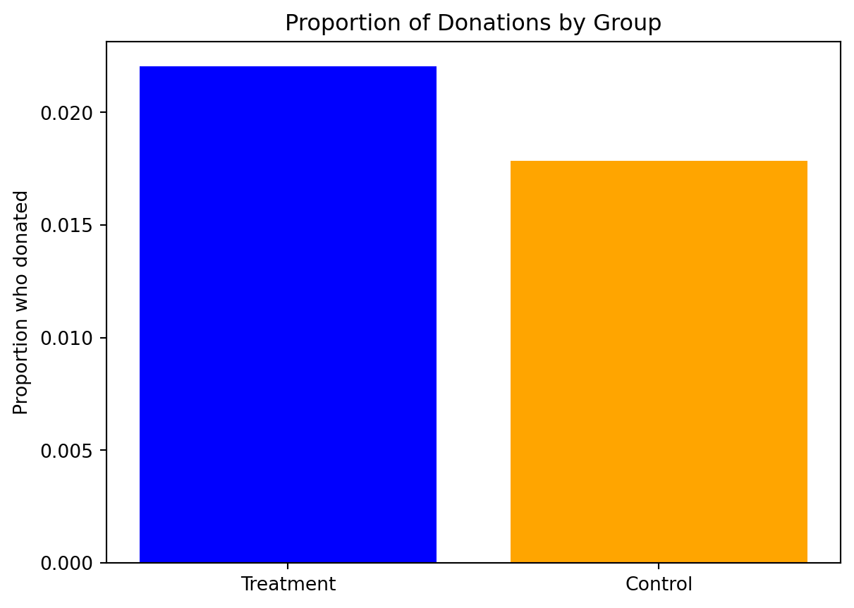

As visual, we can interpret that the treatment group had a higher response rate for making donations than the control group, which implies that the treatment might have effective in encouraging donations. However, we have to do further statistical analysis to assess the reliability of this observed difference

T-test

First of all, let’s check the similarity between our data and Panel A in table 2A

Code

donated_treatment = data[data['treatment'] == 1]['gave']
donated_control = data[data['treatment'] == 0]['gave']

x_bar_treatment = donated_treatment.mean()
x_bar_control = donated_control.mean()
print(f'The response rate of treatment group panel A is {round(x_bar_treatment, 3)}')
print(f'The response rate of treatment group panel A is {round(x_bar_control, 3)}')

The response rate of treatment group panel A is 0.022
The response rate of treatment group panel A is 0.018

Code

# Apply the t_values function that we defined above
t_value_donated = t_value(donated_treatment, donated_control)
print(f"T_value is {round(t_value_donated, 3)}")

T_value is 3.209

Code

#Apply the degree of freedom funcion that we defined above
dof_donated = dof(donated_treatment, donated_control)
print(f"Degree of freedom is {round(dof_donated, 2)}")

Degree of freedom is 36576.84

Code

# Find p-value
p_value = (1 - t.cdf(t_value_donated, dof_donated))*2
print(f"P_value is {round(p_value, 3)}")

P_value is 0.001

The independent t-test on the ‘gave’ variable between the treatment and control groups yields a t-statistic of approximately 3.209 and a p-value of 0.001.

This p-value is less than the alpha level of 0.05, indicating that there is a statistically significant difference between the treatment and control groups in terms of the proportion of participants who made a donation.

Linear Regression

Code

lr = rsm.model.regress(
    data = data,
    rvar = 'gave',
    evar = 'treatment'
)
lr.coef.round(3)

	index	coefficient	std.error	t.value	p.value
0	Intercept	0.018	0.001	16.225	0.000	***
1	treatment	0.004	0.001	3.101	0.002	**

The linear regression results are as follows:

The coefficient for treatment is approximately 0.004 with a standard error of about 0.001.
The t-statistic for the treatment coefficient is 3.1, and the p-value is 0.002.

This p-value is also less than the alpha level of 0.05, suggesting that the treatment has a statistically significant effect on the likelihood of making a donation. The positive coefficient indicates that being in the treatment group is associated with higher odds of giving a donation compared to the control group.

Both the t-test and logistic regression demonstrate that there is a significant difference in the donation behavior between the treatment and control groups, with the treatment group showing a higher propensity to give

In the context of the experiment, the statistical significance of the treatment group’s coefficient implies that the treatment has a positive effect on the likelihood that someone will donate. This insight into human behavior suggests that the strategy employed to encourage donations in the treatment group was effective in increasing donation rates.

In other words, if the experiment involved sending out letters asking for donations, and the treatment group received letters with a special message or offer not given to the control group, we could interpret these results to mean that the special message or offer motivated more people to donate. The important takeaway here is that small changes in how we ask for donations can have a significant impact on people’s willingness to contribute to a cause. This aligns with the findings presented in Table 2A, Panel A, which we aimed to confirm with our analysis.

Probit Regression

Code

X_linear = sm.add_constant(data['treatment'])  # Add a constant to the independent variable
y_linear = data['gave'] 
# Fit the Probit regression model using 'treatment' as the predictor and 'gave' as the binary outcome
probit_model = sm.Probit(y_linear, X_linear).fit()

# Get the summary of the Probit regression results
probit_summary = probit_model.summary()
# Extract only the regression results table
probit_results_table = probit_summary.tables[1]

# To display or print out the table
print(probit_results_table)

Optimization terminated successfully.
         Current function value: 0.100443
         Iterations 7
==============================================================================
                 coef    std err          z      P>|z|      [0.025      0.975]
------------------------------------------------------------------------------
const         -2.1001      0.023    -90.073      0.000      -2.146      -2.054
treatment      0.0868      0.028      3.113      0.002       0.032       0.141
==============================================================================

The Probit regression results are as follows:

The coefficient for treatment is 0.0868, with a standard error of 0.028. The z-statistic for the treatment coefficient is 3.113, and the p-value is 0.002.

The coeficient and standard errors do not match between the Table 3 on the paper and the Probit Regression, it matches to the Linear regression results instead

However, p value of both models are the same, which is smaller than 0.05, sugessts that treatment had a positive impact on the probability of giving, which supports the same notion: the treatment apprears to have effectively encouraged more people to donate

Differences between Match Rates

The Z score formula of proportion is \[ z = \frac{p_a - p_b}{\sqrt{\frac{p_a(1 - p_a)}{n_a} + \frac{p_b(1 - p_b)}{n_b}}} \]

Same as the t_value function above, let’s define z_score function

Code

def z_score(data1, data2, full_data):
    p1 = data1.mean()
    p2 = data2.mean()

    numerator = p1-p2
    denominator = np.sqrt((p1*(1-p1))/len(data1) + (p2*(1-p2)/len(data2)))

    z_score = numerator / denominator
    return z_score

Double check the similarity response rate to Table 2 Panel A

Code

gave_ratio1 = data[data['ratio'] == 1]['gave']
gave_control = data[data['ratio'] == "Control"]['gave']
gave_ratio2 = data[data['ratio'] == 2]['gave']
gave_ratio3 = data[data['ratio'] == 3]['gave']

print(f'Response rate of 1:1 matching is {round(gave_ratio1.mean(), 3)}')
print(f'Response rate of 2:1 matching is {round(gave_ratio2.mean(), 3)}')
print(f'Response rate of 3:1 matching is {round(gave_ratio3.mean(), 3)}')

Response rate of 1:1 matching is 0.021
Response rate of 2:1 matching is 0.023
Response rate of 3:1 matching is 0.023

Control vs 1:1 match

\[H_0: p_{Control} = p_{1:1\;Ratio}\] \[H_a: p_{Control} \neq p_{1:1\;Ratio}\]

Z-test

Code

# Apply the function that we defined above
z_score_ratio1 = z_score(gave_ratio1, gave_control, data)
print(f'Z score is {round(z_score_ratio1, 3)}')

Z score is 1.705

Code

# find p value
p_value = norm.sf(z_score_ratio1)*2
print(f"p_value is {round(p_value, 3)}")

p_value is 0.088

Z-Value: A z-value of 1.705 indicates that the effect of being in the 1:1 match ratio group is 1.705 standard deviations away from the mean effect of being in the control group. This suggests a positive direction of influence towards increasing the likelihood of donation.

P-Value: The p-value of 0.088, though close, is above the conventional threshold of 0.05 (95% confidence level). This suggests that while there is some evidence to suggest an effect, it does not meet the usual criteria for statistical significance. Hence, we would not reject the null hypothesis at the 5% significance level, which states there is no difference in donation likelihood between the 1:1 match and control groups

Control vs 2:1 match

\[H_0: p_{Control} = p_{2:1\;Ratio}\] \[H_a: p_{Control} \neq p_{2:1\;Ratio}\]

Z-test

Code

z_score_ratio2 = z_score(gave_ratio2, gave_control, data)
print(f'Z score is {round(z_score_ratio2, 4)}')

Z score is 2.7397

Code

# find p value
p_value = norm.sf(z_score_ratio2)*2
print(f"p_value is {round(p_value, 3)}")

p_value is 0.006

Z-Value: A z-value of 2.739 indicates that the effect of being in the 2:1 match ratio group is 2.739 standard deviations away from the mean effect of being in the control group. This represents a stronger and more distinct effect compared to the control, suggesting a significant positive influence on donation likelihood.

P-Value: The p-value of 0.006 is well below the conventional threshold of 0.05, indicating strong statistical significance. This suggests that we can reject the null hypothesis, or there is significant difference in the likelihood of making a donation between the 2:1 match ratio and control groups.

Control vs 3:1 match

\[H_0: p_{Control} = p_{3:1\;Ratio}\] \[H_a: p_{Control} \neq p_{3:1\;Ratio}\]

Z-test

Code

z_score_ratio3 = z_score(gave_ratio3, gave_control, data)
print(f'Z score is {round(z_score_ratio3, 3)}')

Z score is 2.793

Code

# find p value
p_value = norm.sf(z_score_ratio3)*2
print(f"p_value is {round(p_value, 3)}")

p_value is 0.005

Z-Value: A z-value of 2.793 indicates that the effect of being in the 3:1 match ratio group is nearly 2.8 standard deviations away from the mean effect of being in the control group. This shows a strong positive impact of the 3:1 matching offer on the likelihood of making a donation.

P-Value: The p-value of 0.0052 clearly falls below the typical significance threshold of 0.05, affirming that this result is statistically significant. This strongly suggests rejecting the null hypothesis, or there is significant difference in donation likelihood between the 3:1 match ratio and the control groups.

About the figures suggest

Support the statement: If the match thresholds for different ratios were relatively low and thus easilu attainable, and the data still shows a significant different between higher ratios and the control, it supports the notion that increasing the match ratio is an effectve strategy. It suggests that the actual ratio, rather than the ease of achieving a match, motivates donors
Contradiction of the statement: The significant effects effects observed at higher match ratios contradict any implication the match ratios do not influence donor behavior. It shows that higher ratios can indeed motivate more donations

Regression on ratio1, ratio2, ratio3

First of all, create a new ratio1 variable

Code

data['ratio1'] = rsm.ifelse(data.ratio == 1, 1, 0)

Linear regression

Code

lr = rsm.model.regress(
    data = data,
    rvar = 'gave',
    evar = ['ratio1', 'ratio2', 'ratio3']
)
lr.coef.round(3)

	index	coefficient	std.error	t.value	p.value
0	Intercept	0.018	0.001	16.225	0.000	***
1	ratio1	0.003	0.002	1.661	0.097	.
2	ratio2	0.005	0.002	2.744	0.006	**
3	ratio3	0.005	0.002	2.802	0.005	**

The linear regression results are as follows:

ratio1 represent 1:1 matching:

Coefficient: 0.003: suggesting that ratio increases the probability of making a donation by 0.3% points
p_value = 0.097

At the 95% confidence level, the coefficient for 1:1 match ratio is not statistically significant because p_value is greater than 0.05, which means we are less confident that 1:1 match ratio has a real effect on the donation probability in the population

ratio2 represent 2:1 matching:

Coefficient: 0.005, indicates a 0.5% point increase in the probability of making a donation
P-value: 0.006

The coefficient for the 2:1 match ratio is statistically significant at the 95% confidence level, as the p-value is well below 0.05, which means we can quite confident that the 2:1 match ratio has a positive effect on the probability of donating

ratio3 represent 3:1 matching:

Coefficient: 0.005, also indicates a 0.5% point increase in the probability of making a donation
P-value: 0.005

Similarly, the coefficient for the 3:1 match ratio is statistically significant at the 95% confidence level.

Statistical Precision

The ‘std.error’ column shows the standard error of each coefficient, which is a measure of the precision of the coefficient estimate. Smaller standard errors indicate more precise estimates. In this table, the standard errors for the treatment levels are the same (0.002), suggesting similar levels of precision across these estimates.

The results indicate that only the 2:1 and 3:1 match ratios significantly increase the likelihood of donations compared to the control group at the 95% confidence level. The effects of these higher match ratios are robust, suggesting that they are effective strategies for increasing donation rates.

The 1:1 match ratio, while showing a positive effect, does not reach the threshold for statistical significance at this confidence level. This implies that while there might be a slight increase in donation likelihood with a 1:1 match, the evidence is not strong enough to conclusively state this at the 95% confidence level.

Response rate difference

Code

rr_1_1 = data[data['ratio1'] == 1]['gave'].mean()
rr_2_1 = data[data['ratio2'] == 1]['gave'].mean()
rr_3_1 = data[data['ratio3'] == 1]['gave'].mean()

rr_diff_11_vs_21 = rr_2_1 - rr_1_1
rr_diff_21_vs_31 = rr_3_1 - rr_2_1

print(f'The response rate difference between the 1:1 and 2:1 match ratios {round(rr_diff_11_vs_21, 3)}')
print(f'The response rate difference between the 2:1 and 3:1 match ratios {round(rr_diff_21_vs_31, 3)}')

The response rate difference between the 1:1 and 2:1 match ratios 0.002
The response rate difference between the 2:1 and 3:1 match ratios 0.0

Recall the linear regression result above:

Code

lr.coef.round(3)

	index	coefficient	std.error	t.value	p.value
0	Intercept	0.018	0.001	16.225	0.000	***
1	ratio1	0.003	0.002	1.661	0.097	.
2	ratio2	0.005	0.002	2.744	0.006	**
3	ratio3	0.005	0.002	2.802	0.005	**

Code

coef_ratio1 = 0.003
coef_ratio2 = 0.005
coef_ratio3 = 0.005

coef_11_vs_21 = coef_ratio2 - coef_ratio1
coef_21_vs_31 = coef_ratio3 - coef_ratio2

print(f'The response rate difference between the 1:1 and 2:1 match ratios from regression is {round(coef_11_vs_21, 3)}')
print(f'The response rate difference between the 2:1 and 3:1 match ratios from regression is {round(coef_21_vs_31, 3)}')

The response rate difference between the 1:1 and 2:1 match ratios from regression is 0.002
The response rate difference between the 2:1 and 3:1 match ratios from regression is 0.0

1:1 vs 2:1 : The very small difference (0.002) suggests only a marginal improvement in the response rate from the 1:1 and 2:1 match ratio. This indicates that while the 2:1 match ratio might be slightly more effective than 1:1, the difference is minimal

2:1 vs 3:1 The zero difference suggest that there is no additional benefit in increasing the match ratio from 2:1 to 3:1 regarding the likelihood of donations. This suggests diminishing returns when the match ratio increase beyond 2:1

These findings imply that while increasing the match ratio from 1:1 to 2:1 might offer a slight increase in donation likelihood, increasing it further to 3:1 does not yield additional benefits. This could be crucial for organizations in deciding how aggressively to pursue higher matching ratios in their fundraising strategies. The minimal differences suggest that other factors may be more critical in influencing donation behavior than merely adjusting the match ratio.

Size of Charitable Contribution

\[H_0: \mu_{amount\;treatment} = \mu_{amount\;control} \] \[H_a: \mu_{amount\;treatment} \neq \mu_{amount\;control} \]

Code

amount_treatment = data.loc[data['treatment'] == 1,'amount']
amount_control = data.loc[data['treatment'] == 0,'amount']

# Apply the t_values function that we defined above
t_value_amount = t_value(amount_treatment, amount_control)
print(f"T_value is {t_value_amount}")

T_value is 1.9182617883567805

Code

#Apply the degree of freedom funcion that we defined above
dof_amount = dof(amount_treatment, amount_control)
print(f"Degree of freedom is {dof_amount}")

Degree of freedom is 36216.06015374612

Code

# Find p-value
p_value = (1-t.cdf(t_value_amount, dof_amount))*2
print(f"P_value is {p_value}")

P_value is 0.055085678607487365

The t-test results show a t-statistic of approximately 1.918 with a p-value of 0.055. This p-value is slightly above the conventional threshold of 0.05, indicating that the difference in average donation amounts between the treatment and control groups is not statistically significant at the 5% level. However, the p-value is close to the threshold, suggesting a potential trend where the treatment group might have higher donation amounts than the control group, though this difference isn’t strong enough to be considered statistically significant.

Linear Regression

Code

lr = rsm.model.regress(
    data = data,
    rvar = 'amount',
    evar = 'treatment'
)
lr.coef.round(3)

	index	coefficient	std.error	t.value	p.value
0	Intercept	0.813	0.067	12.063	0.000	***
1	treatment	0.154	0.083	1.861	0.063	.

Linear Regression Results:

Intercept: 0.8133

This suggests that the average donation amount for the control group is approximately 0.813 units.

Coefficient for Treatment: 0.154

This indicates that being in the treatment group is associated with an increase in the donation amount by approximately 0.154 units compared to the control group.

P-Value for Treatment: 0.063

The p-value is slightly above the conventional threshold of 0.05, indicating that the effect of treatment on donation amount is not statistically significant at the 5% level. However, it’s close, suggesting a potential positive impact of the treatment on donation amounts.

Overall Interpretation: Both the t-test and the linear regression suggest that the treatment might have a slight positive effect on donation amounts, but this effect does not reach statistical significance. This could imply that while the treatment potentially influences donations positively, the effect is not large or consistent enough across the sample to conclude definitively about its effectiveness. It’s also possible that other variables not considered here could be influencing the donations, and including those in the model could potentially change these results.

Limit only those who made a donation:

Code

data_donated = data[data['amount'] > 0]

T-Test

Code

donated_treatment = data_donated.loc[data_donated['treatment'] == 1,'amount']
donated_control = data_donated.loc[data_donated['treatment'] == 0,'amount']

# Apply the t_values function that we defined above
t_value_donated = t_value(donated_treatment, donated_control)
print(f"T_value is {t_value_donated}")

T_value is -0.5846089783693985

Code

#Apply the degree of freedom funcion that we defined above
dof_donated = dof(donated_treatment, donated_control)
print(f"Degree of freedom is {dof_donated}")

Degree of freedom is 557.4599283248195

Code

# Find p-value
p_value = t.cdf(t_value_donated, dof_donated)*2
print(f"P_value is {p_value}")

P_value is 0.5590471873269819

The t-statistic of -0.5846 suggests a lower average donation amount in the treatment group compared to the control group among donors, though the difference is minor.

The p-value of 0.559 indicates that this difference is not statistically significant. This means we do not have sufficient evidence to conclude that the treatment affects donation amounts among those who donate.

Linear Regression

Code

lr = rsm.model.regress(
    data = data_donated,
    rvar = 'amount',
    evar = 'treatment'
)
lr.coef.round(3)

	index	coefficient	std.error	t.value	p.value
0	Intercept	45.540	2.423	18.792	0.000	***
1	treatment	-1.668	2.872	-0.581	0.561

Treatment Coefficient: The coefficient for the treatment group is approximately -1.67 with a standard error of about 2.87. This suggests that, on average, the treatment group donated about 1.67 units less than the control group among those who donated.

Statistical Significance: P-value for the Treatment: The p-value for the treatment effect is 0.561, which is not statistically significant. This implies that there is no strong evidence to suggest that the treatment effect differs from zero in the population of donors.

The negatice coefficient for the treatment group suggests that the treatment potentially lead to a decrease in the amount donated compared to the control group among those who donated. However, the lack of statistical significance (p-value > 0.05) means we can not confidently assert that this treatment effect is different from zero in the broader donor population.

Causal Interpretation:

Whether the treatment coefficient can be interpreted causally depends on how the treatment was assigned. If the treatment was randomly assigned to participants, then the coefficient could potentially have a causal interpretation. Random assignment would help control for both observed and unobserved confounding variables, allowing us to attribute differences in outcomes directly to the treatment effect.

What Did We Learn?

The analysis indicates that among those who chose to donate, the treatment did not significantly increase donation amounts. In fact, the point estimate suggests a slight decrease in donations, but this result is not statistically significant. This finding helps understand the treatment’s impact specifically on the subset of the population that decides to donate, complementing the broader analysis which includes non-donors.

Plots

Code

# Prepare the plots for treatment and control groups who made donations
fig, axes = plt.subplots(nrows=1, ncols=2, figsize=(14, 6))

# Plot for Treatment Group
axes[0].hist(donated_treatment, bins=30, color='blue', alpha=0.7)
axes[0].axvline(donated_treatment.mean(), color='red', linestyle='dashed', linewidth=1)
axes[0].set_title('Treatment Group Donation Amounts')
axes[0].set_xlabel('Donation Amount')
axes[0].set_ylabel('Frequency')
axes[0].text(donated_treatment.mean(), max(axes[0].get_ylim()) * 0.5, f'Average: {donated_treatment.mean():.2f}', color='red')

# Plot for Control Group
axes[1].hist(donated_control, bins=30, color='green', alpha=0.7)
axes[1].axvline(donated_control.mean(), color='red', linestyle='dashed', linewidth=1)
axes[1].set_title('Control Group Donation Amounts')
axes[1].set_xlabel('Donation Amount')
axes[1].set_ylabel('Frequency')
axes[1].text(donated_control.mean(), max(axes[1].get_ylim()) * 0.5, f'Average: {donated_control.mean():.2f}', color='red')

plt.tight_layout()
plt.show()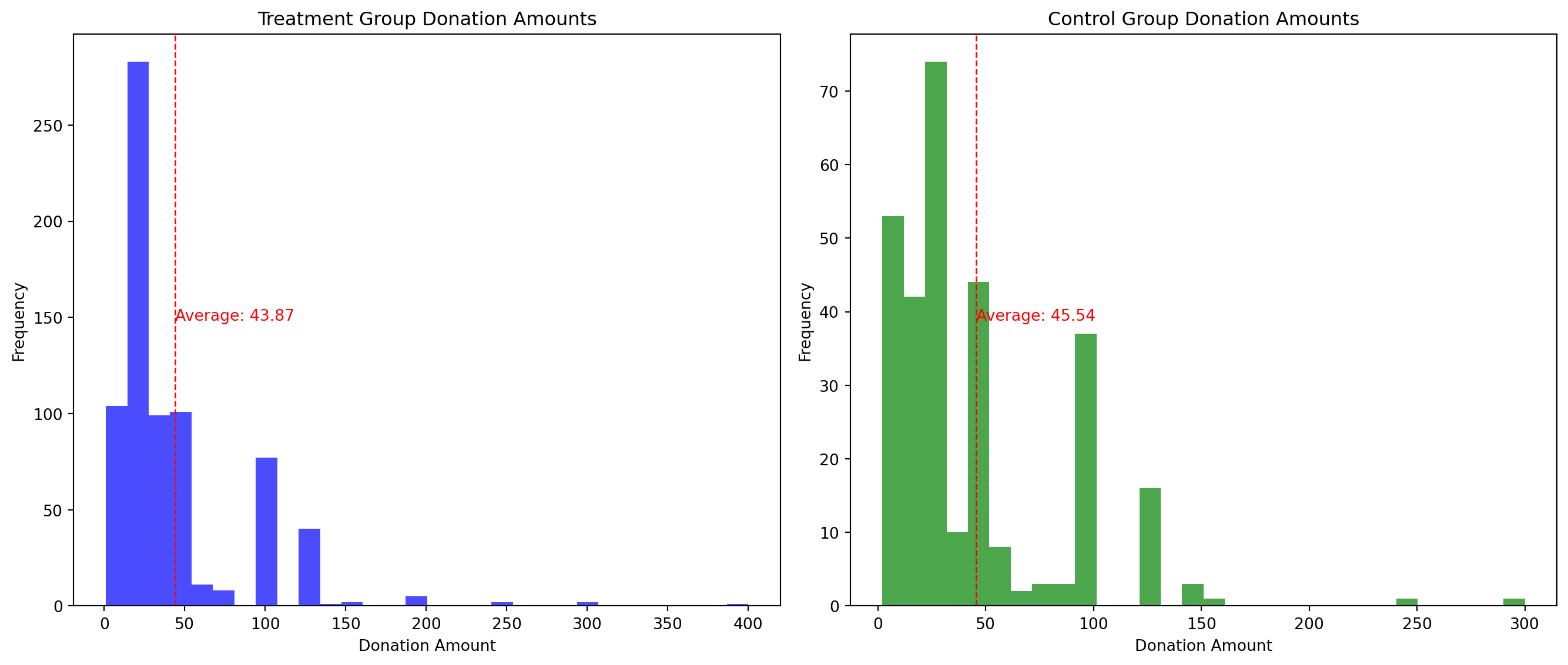

Treatment Group Donation Amounts:

The majority of donations are concentrated in the lower range of amounts, with the frequency decreasing as the amount increases.

There’s a significant frequency at the lowest amount, indicating that many donations are of a small value.

The average donation amount in the treatment group is indicated by a vertical dotted red line and is annotated as $43.87.

Control Group Donation Amounts:

Similar to the treatment group, most donations are of a lower amount, with frequency tapering off for higher donation amounts.

The distribution of donations appears slightly more spread out than the treatment group, with some higher amounts being more frequent compared to the treatment group.

The average donation amount for the control group is slightly higher than the treatment group, marked by a vertical dotted red line, at $45.54.

Interpretation:

The control group has a slightly higher average donation amount compared to the treatment group.
Both histograms appear right-skewed, which is common in financial data since a large number of small donations are often accompanied by a smaller number of much larger donations

Simulation Experiment

Law of Large Numbers

Code

# Define probabilities for Bernoulli distributions
p_control = 0.018  # Probability for control group
p_treatment = 0.022  # Probability for treatment group

# Simulate 100,000 draws for the control group
control_samples = np.random.binomial(1, p_control, 100000)

# Simulate 10,000 draws for the treatment group
treatment_samples = np.random.binomial(1, p_treatment, 10000)

# Calculate differences for each of the first 10,000 elements in the control sample (to match treatment sample size)
differences = treatment_samples - control_samples[:10000]

# Calculate cumulative averages of differences
cumulative_averages = np.cumsum(differences) / (np.arange(10000) + 1)

# Plot the cumulative averages of the differences
plt.figure(figsize=(10, 6))
plt.plot(cumulative_averages, label='Cumulative Average of Differences', color='blue')
plt.axhline(y=(p_treatment - p_control), color='red', linestyle='dashed', label='True Difference (0.022 - 0.018)')
plt.xlabel('Number of Simulations')
plt.ylabel('Cumulative Average of Difference')
plt.title('Cumulative Average of Differences Between Treatment and Control')
plt.legend()
plt.grid(True)
plt.show()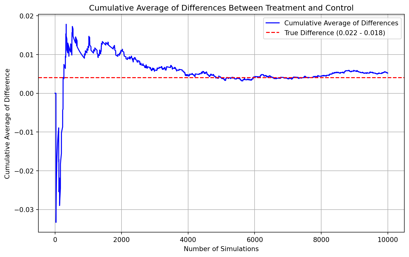

Explaination of the plot The plot above illustrates the cumulative average of differences in donation behavior between treatment group (with a charitable donation match) and the control group (without a match), based on simulated data.

Blue line: This represents the cumulative average of the difference between the donation outcomes of indiividual in the treatmetn and control groups across 10,000 simulated trial. The differences are calculated for each trial as the outcome of the treatment minus the outcome of the control.
Red dashed line: This line marks the true difference in means between the probabilities of making a donation in the treatment and control groups, which is p_treatment - p_control = 0.022 - 0.018 = 0.004.

Observations from the plot

The blue line, or the cumulative average of differences, fluctuates initially but starts to stabilize and approach the red dashed line as the number of trials increases. This behavior exemplifies the Law of Large Numbers, which states that as the number of trials increases, the sample average will converge to the expected value (in this case, the true difference in means).

The plot confirms that with a sufficient number of trials, the cumulative average of the differences in donation behavior between the treatment and control groups approaches the true difference in means. This simulation reinforces our understanding of statistical concepts like the Law of Large Numbers and provides a visual affirmation that with enough data, our estimates can reliably approximate true population parameters. This also supports the validity of using such statistical methods to evaluate the effects of interventions like charitable donation matches

Central Limit Theorem

Code

# Define sample sizes to simulate
sample_sizes = [50, 200, 500, 1000]

fig, axes = plt.subplots(nrows=1, ncols=4, figsize=(20, 5), sharey=True)

# Simulate the process and plot the histograms
for i, sample_size in enumerate(sample_sizes):
    # Simulate drawing samples and calculating the means 1000 times
    sample_means = np.array([np.mean(np.random.binomial(1, p_treatment, sample_size) - 
                                     np.random.binomial(1, p_control, sample_size)) 
                             for _ in range(1000)])
    
    # Plot the histogram
    axes[i].hist(sample_means, bins=30, orientation='horizontal', color='blue', alpha=0.6, edgecolor='black')
    
    # Calculate the mean and standard deviation for the normal distribution curve
    mean_of_sample_means = np.mean(sample_means)
    std_dev_of_sample_means = np.std(sample_means)

    # Generate values for the normal distribution curve
    curve_x = np.linspace(mean_of_sample_means - 3 * std_dev_of_sample_means, 
                          mean_of_sample_means + 3 * std_dev_of_sample_means, 100)
    curve_y = (1 / (std_dev_of_sample_means * np.sqrt(2 * np.pi)) *
               np.exp(-(curve_x - mean_of_sample_means) ** 2 / (2 * std_dev_of_sample_means ** 2)))
    
    # Scale the curve y to match the histogram scale
    curve_y_scaled = curve_y * max(np.histogram(sample_means, bins=30)[0]) / max(curve_y)
    
    # Draw the normal distribution curve as a red line
    axes[i].plot(curve_y_scaled, curve_x, '-')

    # Add a red dashed line at the true difference
    axes[i].axhline(y=0.004, color='red', linestyle='dashed', linewidth=2)

    # Set titles and labels
    axes[i].set_title(f'Sample Size {sample_size}')
    axes[i].set_xlabel('Frequency' if i == len(sample_sizes) - 1 else '')  # Only add xlabel to the last subplot
    axes[i].set_ylabel('Average Difference' if i == 0 else '')  # Only add ylabel to the first subplot

# Adjust layout for better fit
plt.tight_layout()

# Show the plot
plt.show()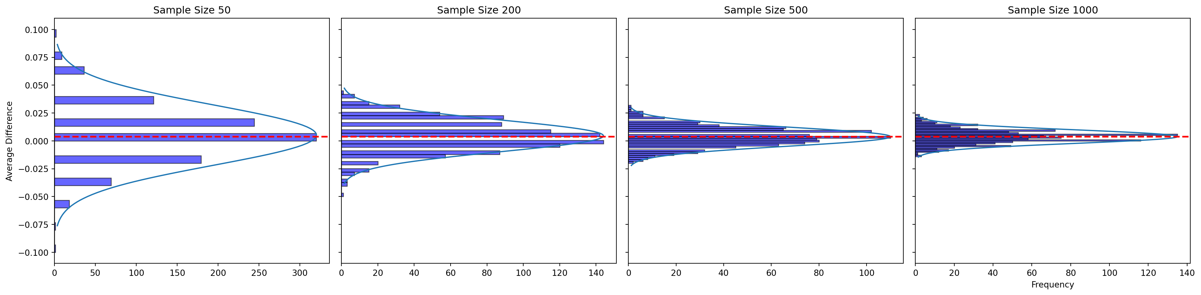

As we can see:

Sample Size 50: There is considerable variability around the true difference, indicating that smaller sample sizes can produce estimates that fluctuate widely.

Sample Size 200: The histogram becomes tighter around the true difference, with less variability than the sample size of 50.

Sample Size 500: Further reduction in variability is observed, and the distribution of averages is centered closely around the true difference.

Sample Size 1000: This histogram shows the least variability, and the average differences are clustering tightly around the true difference, with the center of the distribution aligning closely with the red line.

Law of Large Numbers: As the sample size increases, the cumulative average difference becomes more consistent and stable around the true difference. This is a demonstration of the Law of Large Numbers—the sample averages converge to the expected value as the sample size grows.

Central Limit Theorem: As the sample size increases, the distribution of sample means (average differences in this case) becomes more symmetrical and bell-shaped, which is evidence of the Central Limit Theorem in action. The sample means for larger sample sizes tend to form a normal distribution centered around the true population mean.

Zero in the Distribution: In all histograms, the zero mark is not in the middle of the distribution; it’s in the left tail. This is because the treatment group has a higher probability of donating than the control group (0.022 vs. 0.018), so the true difference is expected to be positive (0.004), not zero.